Bundle: Introduction to Statistics and Data Analysis, 5th + WebAssign Printed Access Card: Peck/Olsen/Devore. 5th Edition, Single-Term
5th Edition
ISBN: 9781305620711
Author: Roxy Peck, Chris Olsen, Jay L. Devore
Publisher: Cengage Learning
expand_more
expand_more
format_list_bulleted
Concept explainers
Videos
Textbook Question
Chapter 13.3, Problem 30E
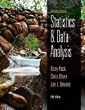
The article “Vital Dimensions in Volume Perception: Can the Eye Fool the Stomach?” (Journal of Marketing Research [1999]: 313–326) gave the accompanying data on the dimensions of 27 representative food products (Gerber baby food, Cheez Whiz, Skippy Peanut Butter, and Ahmed’s tandoori paste, to name a few).
- a. Fit the simple linear regression model that would allow prediction of the maximum width of a food container based on its minimum width.
- b. Calculate the standardized residuals (or just the residuals if a computer program that doesn’t give standardized residuals is used) and make a residual plot to determine whether there are any outliers.
- c. The data point with the largest residual is for a 1-liter Coke bottle. Delete this data point and determine the equation of the regression line. Did deletion of this point result in a large change in the equation of the estimated regression line?
- d. For the regression line of Part (c), interpret the estimated slope and, if appropriate, the intercept.
- e. For the data set with the Coke bottle deleted, are the assumptions of the simple linear regression model reasonable? Give statistical evidence.
Expert Solution & Answer

Trending nowThis is a popular solution!

Students have asked these similar questions
1. Regression methods were used to analyze the data from a study investigating the relationship between roadway surface temperature (x) and pavement deflection ( y). Summary quantities were n = 20, ∑ y i = 12.75, ∑ y i 2 = 8.86, ∑ x i = 1478, ∑ x i 2 = 143 , 215.80, and ∑ x i y i = 1083.67.
(a) Calculate the least squares estimates of the slope and intercept. Graph the regression line. with plotting of graph(b) Use the equation of the fitted line to predict what pavement deflection would be observed when the surface temperature is 85F.(c) What is the mean pavement deflection when the surface temperature is 90F?
2. A botanist is willing to understand the relation between volume, girth and height of black cherry trees.
To this end, she collects data that is presented in trees table of the datasets library. Build a predictive
multiple linear regression model for volume using girth and height as independent variables.
a. What does the F-test tell about the model? Explain the result using the null hypothesis of the
test.
b. Provide confidence and prediction intervals for a black cherry tree with 10 inch of girth and 82
feet tall.
The rental of an apartment (R) near campus is a function of the square
footage (Sq). A random sample of apartments near campus yielded the
following summary statistics:
R= $350, Sq = 100, sR = $ 30, and 8 są = 10. Suppose also that the
correlation between price and weight is 0.8.
(a) Write the implied least squares linear regression equation.
(b) Suppose an apartment has 75 sqft. Predict its price based on the
above model.
(c) Suppose the true rental of the apartment in part (b) is $ 325. What is
the value of the residual?
Chapter 13 Solutions
Bundle: Introduction to Statistics and Data Analysis, 5th + WebAssign Printed Access Card: Peck/Olsen/Devore. 5th Edition, Single-Term
Ch. 13.1 - Prob. 1ECh. 13.1 - The flow rate in a device used for air quality...Ch. 13.1 - The paper Predicting Yolk Height, Yolk Width,...Ch. 13.1 - Prob. 4ECh. 13.1 - Suppose that a simple linear regression model is...Ch. 13.1 - a. Explain the difference between the line y x...Ch. 13.1 - Prob. 7ECh. 13.1 - Hormone replacement therapy (HRT) is thought to...Ch. 13.1 - Prob. 9ECh. 13.1 - A simple linear regression model was used to...
Ch. 13.1 - Consider the accompanying data on x = Advertising...Ch. 13.2 - What is the difference between and b? What is the...Ch. 13.2 - The largest commercial fishing enterprise in the...Ch. 13.2 - Prob. 14ECh. 13.2 - Prob. 15ECh. 13.2 - Prob. 16ECh. 13.2 - An experiment to study the relationship between x...Ch. 13.2 - The paper The Effects of Split Keyboard Geometry...Ch. 13.2 - The authors of the paper Decreased Brain Volume in...Ch. 13.2 - Do taller adults make more money? The authors of...Ch. 13.2 - Researchers studying pleasant touch sensations...Ch. 13.2 - Prob. 22ECh. 13.2 - Prob. 23ECh. 13.2 - Consider the accompanying data on x = Research and...Ch. 13.2 - Prob. 25ECh. 13.2 - In anthropological studies, an important...Ch. 13.3 - The graphs accompanying this exercise are based on...Ch. 13.3 - Prob. 28ECh. 13.3 - Prob. 29ECh. 13.3 - The article Vital Dimensions in Volume Perception:...Ch. 13.3 - Prob. 31ECh. 13.3 - An investigation of the relationship between x =...Ch. 13.4 - Prob. 33ECh. 13.4 - Prob. 34ECh. 13.4 - Prob. 35ECh. 13.4 - Prob. 36ECh. 13.4 - A subset of data read from a graph that appeared...Ch. 13.4 - Prob. 38ECh. 13.4 - Prob. 39ECh. 13.4 - Prob. 40ECh. 13.4 - The shelf life of packaged food depends on many...Ch. 13.4 - For the cereal data of the previous exercise, the...Ch. 13.4 - The article Performance Test Conducted for a Gas...Ch. 13.5 - Prob. 44ECh. 13.5 - Prob. 45ECh. 13.5 - A sample of n = 353 college faculty members was...Ch. 13.5 - Prob. 47ECh. 13.5 - Prob. 48ECh. 13.5 - The accompanying summary quantities for x =...Ch. 13.5 - Prob. 50ECh. 13.5 - Prob. 51ECh. 13.6 - Prob. 52ECh. 13 - Prob. 53CRCh. 13 - Prob. 54CRCh. 13 - Prob. 55CRCh. 13 - The article Photocharge Effects in Dye Sensitized...Ch. 13 - Prob. 57CRCh. 13 - Prob. 58CRCh. 13 - Prob. 59CRCh. 13 - Prob. 60CRCh. 13 - Prob. 61CRCh. 13 - The article Improving Fermentation Productivity...Ch. 13 - Prob. 63CRCh. 13 - Prob. 64CRCh. 13 - Prob. 65CRCh. 13 - Prob. 1CRECh. 13 - Prob. 2CRECh. 13 - Prob. 3CRECh. 13 - Prob. 4CRECh. 13 - Prob. 5CRECh. 13 - The accompanying graphical display is similar to...Ch. 13 - Prob. 7CRECh. 13 - Prob. 8CRECh. 13 - Consider the following data on y = Number of songs...Ch. 13 - Many people take ginkgo supplements advertised to...Ch. 13 - Prob. 11CRECh. 13 - Prob. 12CRECh. 13 - Prob. 13CRECh. 13 - Prob. 14CRECh. 13 - The discharge of industrial wastewater into rivers...Ch. 13 - Many people take ginkgo supplements advertised to...Ch. 13 - It is hypothesized that when homing pigeons are...Ch. 13 - Prob. 18CRE
Knowledge Booster


Learn more about
Need a deep-dive on the concept behind this application? Look no further. Learn more about this topic, statistics and related others by exploring similar questions and additional content below.Similar questions
- Find the equation of the regression line for the following data set. x 1 2 3 y 0 3 4arrow_forwardThe article "Earthmoving Productivity Estimation Using Linear Regression Techniques" (S. Smith, Journal of Construction Engineering and Management, 1999:133–141) presents the following linear model to predict earth-moving productivity (in m3 moved per hour): Productivity = - 297.877 + 84.787x, + 36.806x, + 151.680x, – 0.081x, – 110.517x5 - 0.267.x, – 0.016x,x, +0.107.x,x5 + 0.0009448x,x, – 0.244x;x, where X1 = number of trucks X2 = number of buckets per load X3 = bucket volume, in m³ X4 = haul length, in m X5 = match factor (ratio of hauling capacity to loading capacity) X6 = truck travel time, in s If the bucket volume increases by 1 m², while other independent variables are unchanged, can you determine the change in the predicted productivity? If so, determine it. If not, state what other information you would need to determine it. b. If the haul length increases by 1 m, can you determine the change in the predicted productivity? If so, determine it. If not, state what other…arrow_forward10. The Shepherd Company's president would like to know the estimated fixed and variable components of a particular cost. Actual data for this cost for four recent periods appear below. Activity Cost Period 1 24 P174 Period 2 25 179 Period 3 20 165 Period 4 22 169 Using the least-squares regression method, what is the cost formula for this cost?arrow_forward
- A magazine publishes restaurant ratings for various locations around the world. The magazine rates the restaurants for food, decor, service, and the cost per person. Develop a regression model to predict the cost per person, based on a variable that represents the sum of the three ratings. The magazine has compiled the accompanying table of this summated ratings variable and the cost per person for 25 restaurants in a major city. Assuming a linear relationship, use the least-squares method to compute the regression coefficients b0 and b1.arrow_forwardCompute the least-squares regression line for predicting the right foot temperature from the left foot temperature. Round the slope and y-Intercept values to four decimal places.arrow_forwardAn article in Technometrics by S. C. Narula and J. F. Wellington (“Prediction, Linear Regression, and a Minimum Sum of Relative Errors,” Vol. 19, 1977) presents data on the selling price (y) and annual taxes (x) for 24 houses. The taxes include local, school and county taxes. The data are shown in the table below. Calculate the least square estimates of slope and intercept. Input answers up to 3 decimal places. Slope = Blank 1 Intercept = Blank 2arrow_forward
- An articie in Technometrics by S.C. Narula and J. F. Wallington Prediction, Lincar Regression, and a Minimum Sum of Relative Errors" Vol. 19, 1977) presents data on the sallingprica (y) and annual taas (x) for 24 houses. The taxes include local, school and county taxes. The data are shown in the following table. Sale Price/1000 Taxas/1000 25.9 4.9176 29.5 5.0208 27.9 4.5429 25.9 4.5573 29.9 5.0597 29.9 3.8910 30.9 5.8980 28.9 5.6039 35.9 5.8282 31.5 5.3003 31.0 6.2712 30.9 5.9592 30.0 5.0500 36.9 8.2464 41.9 6.6969 40.5 7.7841 43.9 9.0384 37.5 5.9894 37.9 7.5422 44.5 8.7951 37.9 6.0831 38.9 8.3607 36.9 8.1400 45.8 9.1416 (a) Calculate the least squares estimates of the slops and intercspt. (Round your answer to 3 decimal places.) (Round your answer to 2 decimal places.) (b) Find the mean selling price given that the taxes paid arex-8.9. (Round your answer to 2 decimal places.)arrow_forward18arrow_forwardWe have data from 209 publicly traded companies (circa 2010) indicating sales and compensation information at the firm-level. We are interested in predicting a company's sales based on the CEO's salary. The variable sales; represents firm i's annual sales in millions of dollars. The variable salary; represents the salary of a firm i's CEO in thousands of dollars. We use least-squares to estimate the linear regression sales; = a + ßsalary; + ei and get the following regression results: regress sales salary . Source Model Residual Total sales salary _cons SS 337920405 2.3180e+10 2.3518e+10 df 1 207 208 Coef. Std. Err. .9287785 .5346574 5733.917 1002.477 MS 337920405 111980203 113066454 t Number of obs F(1, 207) Prob> F R-squared Adj R-squared Root MSE P>|t| 1.74 0.084 5.72 0.000 209 3.02 -.1252934 3757.543 0.0838 0.0144 0.0096 10582 [95% Conf. Interval] 1.98285 7710.291 This output tells us the regression line equation is sales = 5,733.917 +0.9287785 salary. Suppose a CEO of a company…arrow_forward
- The data in the table represent the number of licensed drivers in various age groups and the number of fatal accidents within the age group by gender. Complete parts (a) to (c) below. ..... (a) Find the least-squares regression line for males treating the number of licensed drivers as the explanatory variable, x, and the number of fatal crashes, y, as the response variable. Repeat this procedure for females. Find the least-squares regression line for males. y=x+O Data for licensed drivers by age and gender. (Round the slope to three decimal places and round the constant to the nearest integer as needed.) Find the least-squares regression line for females. x + Number of Number of Number of Male Fatal Number of Female Fatal (Round the slope to three decimal places and round the constant to the nearest integer as needed.) Licensed Drivers Crashes Licensed Drivers Crashes (b) Interpret the slope of the least-squares regression line for each gender, if appropriate. How might an insurance…arrow_forwardA manufacturing firm has developed a skills test, the scores from which can be used to predict workers' production rating factors. (data attached) a. Using POM for Windows' least squares-linear regression module, develop a relationship to forecast production ratings from test scores (round to 3 dec points and use negative signs when necessary) Y = __ + __X where Y=Production rating and X=Test score b. If a worker's test score was 51, what would be your forecast of the worker's production rating? ___ (Enter your response as an integer.) c. Comment on the strength of the relationship between the test scores and production ratings. The coefficient of correlation for the least-squares regression model is ___ and the coefficient of determination is ___.(round to 3 dec places.) There is stong posititive/no/strong negative (choose 1) relationship. The regression equation explains ___% of variation in ratings (integer).arrow_forwardThe weight (in pounds) and height (in inches) for a child were measured every few months over a two-year period. The results are displayed in the scatterplot. The equation ŷ = 17.4 + 0.5x is called the least-squares regression line because it is least able to make accurate predictions for the data. makes the strongest association between weight and height. minimizes the sum of the squared distances from the actual y-value to the predicted y-value. maximizes the sum of the squared distances from the actual y-value to the predicted y-value.arrow_forward
arrow_back_ios
SEE MORE QUESTIONS
arrow_forward_ios
Recommended textbooks for you

 Linear Algebra: A Modern IntroductionAlgebraISBN:9781285463247Author:David PoolePublisher:Cengage Learning
 Elementary Linear Algebra (MindTap Course List)AlgebraISBN:9781305658004Author:Ron LarsonPublisher:Cengage Learning
 Big Ideas Math A Bridge To Success Algebra 1: Stu...AlgebraISBN:9781680331141Author:HOUGHTON MIFFLIN HARCOURTPublisher:Houghton Mifflin Harcourt
 Functions and Change: A Modeling Approach to Coll...AlgebraISBN:9781337111348Author:Bruce Crauder, Benny Evans, Alan NoellPublisher:Cengage Learning
Linear Algebra: A Modern Introduction
Algebra
ISBN:9781285463247
Author:David Poole
Publisher:Cengage Learning
Elementary Linear Algebra (MindTap Course List)
Algebra
ISBN:9781305658004
Author:Ron Larson
Publisher:Cengage Learning
Big Ideas Math A Bridge To Success Algebra 1: Stu...
Algebra
ISBN:9781680331141
Author:HOUGHTON MIFFLIN HARCOURT
Publisher:Houghton Mifflin Harcourt
Functions and Change: A Modeling Approach to Coll...
Algebra
ISBN:9781337111348
Author:Bruce Crauder, Benny Evans, Alan Noell
Publisher:Cengage Learning
Correlation Vs Regression: Difference Between them with definition & Comparison Chart; Author: Key Differences;https://www.youtube.com/watch?v=Ou2QGSJVd0U;License: Standard YouTube License, CC-BY
Correlation and Regression: Concepts with Illustrative examples; Author: LEARN & APPLY : Lean and Six Sigma;https://www.youtube.com/watch?v=xTpHD5WLuoA;License: Standard YouTube License, CC-BY