
Videos
Exercise 34 presented the following data on endotoxin concentration in settled dust both for a sample of urban homes and for a sample of farm homes:
| U: | 6.0 | 5.0 | 11.0 | 33.0 | 4.0 | 5.0 | 80.0 | 18.0 | 35.0 | 17.0 | 23.0 |
| F: | 4.0 | 14.0 | 11.0 | 9.0 | 9.0 | 8.0 | 4.0 | 20.0 | 5.0 | 8.9 | 21.0 |
| 9.2 | 3.0 | 2.0 | 0.3 |
- a. Determine the value of the sample standard deviation for each sample, interpret these values, and then contrast variability in the two samples. [Hint: Σxi = 237.0 for the urban sample and = 128.4 for the farm sample, and
- b. Compute the fourth spread for each sample and compare. Do the fourth spreads convey the same message about variability that the standard deviations do? Explain.
- c. The authors of the cited article also provided endotoxin concentrations in dust bag dust:
| U: | 34.0 | 49.0 | 13.0 | 33.0 | 24.0 | 24.0 | 35.0 | 104.0 | 34.0 | 40.0 | 38.0 | 1.0 |
| F: | 2.0 | 64.0 | 6.0 | 17.0 | 35.0 | 11.0 | 17.0 | 13.0 | 5.0 | 27.0 | 23.0 | |
| 28.0 | 10.0 | 13.0 | 0.2 |
Construct a comparative boxplot (as did the cited paper) and compare and contrast the four samples.
a.
Find and interpret the sample standard deviations of endotoxin concentration of urban homes and farm homes.
Compare the two standard deviations.
Answer to Problem 48E
The sample standard deviation of endotoxin concentration urban homes is
The sample standard deviation of endotoxin concentration of farm homes is
Urban homes have greater variability than farm homes.
Explanation of Solution
Given info:
The data represents the values of endotoxin concentration in settled dust for a sample of urban homes and farm homes. Additional information is that the sum of observations and sum of squares of observations is given for both urban homes and farm homes. The values are
Calculation:
Urban homes:
Variance:
Both the variance and the standard deviation are based on how much each observation deviates from a central point represented by the mean. In general, the greater the distances between the individual observations and the mean, the greater the variability of the data set.
Because the mean acts as a balancing point for observations larger and smaller than it, the sum of the deviations around the mean is always zero.
The shortcut formula for variance is,
The values of sum of observations and sum of squares of observations for urban homes is
The variance of endotoxin concentration of urban homes is:
Thus, the variance of the endotoxin concentration of urban homes is 499.073.
Standard deviation:
The general formula for standard deviation is,
The sample standard deviation of endotoxin concentration of urban homes is:
The standard deviation of endotoxin concentration of urban homes is 22.3.
Interpretation:
The standard deviation is based on how much each observation deviates from a central point represented by the mean.
The standard deviation of endotoxin concentration of urban homes is
From this it can be said that, among 11 observations of endotoxin concentration of urban homes, the approximate deviation between observed endotoxin concentration and mean endotoxin concentration for urban homes is
Farm homes:
The values of sum of observations and sum of squares of observations for farm homes is
The variance of endotoxin concentration of farm homes is:
Thus, the variance of the endotoxin concentration of farm homes is 37.0597.
Standard deviation:
The general formula for standard deviation is,
The sample standard deviation of endotoxin concentration of farm homes is:
The standard deviation of endotoxin concentration of farm homes is 6.0877.
Interpretation:
The standard deviation is based on how much each observation deviates from a central point represented by the mean.
The standard deviation of endotoxin concentration of farm homes is
From this it can be said that among 15 observations of endotoxin concentration of farm homes, the approximate deviation between observed endotoxin concentration and mean endotoxin concentration for farm homes is
Comparison:
The sample standard deviation of endotoxin concentration urban homes is
The sample standard deviation of endotoxin concentration of farm homes is
From the standard deviation of the endotoxin concentration of urban homes and farm homes, it can be concluded that, the variation in observed and mean endotoxin concentration is greater for urban homes than for farm homes.
b.
Obtain the fourth spread of endotoxin concentration in urban homes and farm homes.
Compare the two fourth spreads.
Check whether the interpretation about relative variability of the two different samples is same using standard deviations and fourth spreads are same.
Answer to Problem 48E
The fourth spread of the endotoxin concentration in urban homes is
The fourth spread of the endotoxin concentration in farm homes is
The variation in the endotoxin concentration is higher for urban homes than farm homes.
Yes, standard deviation and fourth spreads convey same message regarding relative variability of endotoxin concentration of urban and farm homes.
Explanation of Solution
Justification:
Fourth spreads:
In contrast to the range, which measures only differences between the extremes, the fourth spread (also called mid spread) is the difference between the upper fourth and the lower fourth. Thus, it measures the variation in the middle 50 percent of the data, and, unlike the range, is not affected by extreme values.
The general formula for fourth spread is,
Fourth spread of urban homes:
The lower fourth, upper fourth and fourth spreads are obtained as follows:
Step1:
The data set is arranged in ascending order as follows:
| S.no | Urban homes |
| 1 | 4 |
| 2 | 5 |
| 3 | 5 |
| 4 | 6 |
| 5 | 11 |
| 6 | 17 |
| 7 | 18 |
| 8 | 23 |
| 9 | 33 |
| 10 | 35 |
| 11 | 80 |
Step2:
The lower fourth of the data is the median of the lower half of the ordered data set.
Here, the values of lower half of the ordered data set are 4, 5, 5, 6, 11and 17.
The number of observations in the lower half of the ordered data set is 6 and is even.
Hence, the median is the average of 3rd and 4th observation of the lower half of the ordered data set.
The lower fourth is obtained below as,
Thus, the lower fourth is 5.5.
Step4:
The upper fourth of the data is the median of the upper half of the ordered data set.
Here, the values of upper half of the ordered data set are 17, 18, 23, 33, 35 and 80.
The number of observations in the upper half of the ordered data set is 6 and is even.
Hence, the median is the average of 3rd and 4th observation of the upper half of the ordered data set.
The upper fourth is obtained below as,
Thus, the upper fourth is 2.015.
Step5:
The lower fourth is 5.5 and the upper fourth is 28.
The fourth spread is obtained below as,
Thus, the fourth spread of urban homes is
Fourth spread of farm homes:
The lower fourth, upper fourth and fourth spreads are obtained as follows:
Step1:
The data set is arranged in ascending order as follows:
| S.no | Farm homes |
| 1 | 0.3 |
| 2 | 2 |
| 3 | 3 |
| 4 | 4 |
| 5 | 4 |
| 6 | 5 |
| 7 | 8 |
| 8 | 8.9 |
| 9 | 9 |
| 10 | 9 |
| 11 | 9.2 |
| 12 | 11 |
| 13 | 14 |
| 14 | 20 |
| 15 | 21 |
Step2:
The lower fourth of the data is the median of the lower half of the ordered data set.
Here, the values of lower half of the ordered data set are 0.3, 2, 3, 4, 4, 5, 8 and 8.9.
The number of observations in the lower half of the ordered data set is 8 and is even.
Hence, the median is the average of 4th and 5th observation of the lower half of the ordered data set.
The lower fourth is obtained below as,
Thus, the lower fourth is 4.
Step4:
The upper fourth of the data is the median of the upper half of the ordered data set.
Here, the values of upper half of the ordered data set are 8.9, 9, 9, 9.2, 11, 14, 20 and 21.
The number of observations in the upper half of the ordered data set is 8 and is even.
Hence, the median is the average of 4th and 5th observation of the upper half of the ordered data set.
The upper fourth is obtained below as,
Thus, the upper fourth is 10.1.
Step5:
The lower fourth is 4 and the upper fourth is 10.1.
The fourth spread is obtained below as,
Thus, the fourth spread of farm homes is
Comparison:
The fourth spread of the urban homes is
The fourth spread of the farm homes is
From the fourth spread of the endotoxin concentration of urban homes and farm homes it can be concluded that, the variation in observed and mean endotoxin concentration is greater for urban homes than for farm homes.
Conclusion:
The standard deviations obtained in part (a) conveyed that, the variability in endotoxin concentration is greater for urban homes than for farm homes.
From these two conclusions, it can be said that the information conveyed by standard deviations and fourth spreads issimilar regarding the variability in endotoxin concentration.
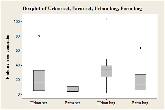
c.
Draw and interpret the comparative boxplot for the four different samples.
Answer to Problem 48E
Box plot:
Output obtained from MINITAB is given below:
Explanation of Solution
Given info:
The data represents the values of endotoxin concentration in dust bag for a sample of urban homes and farm homes.
Calculation:
Box plot:
Software Procedure:
Step-by-step procedure to draw the box plot using the MINITAB software:
- Choose Graph > Box plot.
- Choose Multiple, and then click OK.
- In Graph variables, enter the column of urban-set, farm-set, urban-bag and farm-bag.
- Click OK.
Interpretation:
From the comparativeboxplots, the following points are observed.
- The median endotoxin concentration in bag is higher for urban homes.
- The data sets of settled dust in urban homes, bag dust in urban homes and bag dust in farm homes consist of one outlier each.
- The variation in the entire distribution is lower for the data set of settled dust in urban homes and higher for the data set of bag dust in urban homes.
- Overall it can be concluded that, endotoxin concentration is higher for urban homes than in farm homes for both settled dust and bag dust.
- The overall variation is less for farm homes.
- The bag dust is higher than the settled dust in both urban and farm homes.
Want to see more full solutions like this?
Chapter 1 Solutions
Probability and Statistics for Engineering and the Sciences


- Analysis of several plant-food preparations for potassium ion yielded the following data:arrow_forwardAn article reported data from a study in which both a baseline gasoline mixture and a reformulated gasoline were used. Consider the following observations on age (yr) and NOx emissions (g/kWh): Engine 1 2 3 4 5 6 7 8 9 10 Age 0 0 2 11 7 16 9 0 12 4 Baseline 1.70 4.38 4.06 1.24 5.29 0.59 3.35 3.45 0.73 1.22 Reformulated 1.86 5.91 5.51 2.70 6.50 0.71 4.95 4.86 0.72 1.41 Construct scatter plots of the baseline NOx emissions versus age. What appears to be the nature of the relationship between these two variables? There is no compelling relationship between the data. As age increases, emissions also increase. As age increases, emissions decrease.arrow_forwardPeriodically, the county Water Department tests the drinking water of homeowners for contaminants such as lead and copper. The lead and copper levels in water specimens collected in 1998 for a sample of 10 residents of a subdevelopement of the county are shown below. lead (μμg/L) copper (mg/L) 4.44.4 0.6430.643 2.42.4 0.570.57 1.51.5 0.460.46 2.62.6 0.8950.895 5.95.9 0.20.2 3.43.4 0.540.54 3.83.8 0.2450.245 1.61.6 0.5830.583 5.75.7 0.7690.769 1.71.7 0.2150.215 (a) Construct a 9999% confidence interval for the mean lead level in water specimans of the subdevelopment. ≤μ≤≤μ≤ (b) Construct a 9999% confidence interval for the mean copper level in water specimans of the subdevelopment. ≤μ≤≤μ≤arrow_forward
- rofessor Cornish studied rainfall cycles and sunspot cycles. (Reference: Australian Journal of Physics, Vol. 7, pp. 334-346.) Part of the data include amount of rain (in mm) for 6-day intervals. The following data give rain amounts for consecutive 6-day intervals at Adelaide, South Australia. 7 28 7 1 69 3 1 4 22 7 16 4 54 160 60 73 27 3 3 1 7 144 107 4 91 44 1 8 4 22 4 59 116 52 4 155 42 24 11 43 3 24 19 74 26 63 110 39 34 71 52 39 8 0 15 2 14 9 1 2 4 9 6 10 (i) Find the median. (Use 1 decimal place.)(ii) Convert this sequence of numbers to a sequence of symbols A and B, where A indicates a value above the median and B a value below the median. Test the sequence for randomness about the median at the 5% level of significance. (b) Find the number of runs R, n1, and n2. Let n1 = number of values above the median and n2 = number of values below the median. R n1 n2 (c) In the case, n1 > 20, we cannot use Table 10 of Appendix II to find the critical…arrow_forwardAn article reported data from a study in which both a baseline gasoline mixture and a reformulated gasoline were used. Consider the following observations on age (yr) and NOx emissions (g/kWh): Engine 1 2 3 4 5 6 7 8 9 10 Age 0 0 2 11 7 16 9 0 12 4 Baseline 1.74 4.38 4.04 1.23 5.30 0.58 3.35 3.44 0.73 1.23 Reformulated 1.85 5.93 5.52 2.67 6.54 0.76 4.94 4.87 0.69 1.39 Construct scatter plots of the baseline NOx emissions versus age. Construct scatter plots of the reformulated NOx emissions versus age. What appears to be the nature of the relationship between these two variables? As age increases, emissions also increase.As age increases, emissions decrease. There is no compelling relationship between the data.arrow_forwardQ1 A) List down the measures of central tendency and measures of dispersion 2) The operations manager of a plant that manufactures tires wants to compare the actual inner diameters of two grades of tires, each of B) which is expected to be 575 millimeters. A sample of five tires of each grade was selected, and the results representing the inner diameters of the tires, ranked from smallest to largest, are as follows. Grade X grade Y 568 570 575 578 584 573 574 575 577 578 requirement. a) for each of the tow grades of tries, compute the mwan, median, and standred deviation. b) which grade of tire providing better quality? explain. c) what would be the effect on your answer in (a) and (b) if the last value for grade Y were 588 insert 578 explain. C) The file contins the overall miles per gallon (MPG) OF 2010 family sedan: 24 21 22 23 24 34 34 34 20 20 22 22 44 32 20 20 22 20 39 20 Source:…arrow_forward
- Consider the following measurements of blood hemoglobin concentrations (in g/dL) from three human populations at different geographic locations: population1 = [ 14.7 , 15.22, 15.28, 16.58, 15.10 ] population2 = [ 15.66, 15.91, 14.41, 14.73, 15.09] population3 = [ 17.12, 16.42, 16.43, 17.33] What is the standard error of the difference between the means of population 1 and population 2, needed to calculate the Tukey-Kramer q-statistic? What is the Tukey-Kramer q-statistic for populations 1 and 2? (Report the absolute value, if you get a negative number, multiply by -1)arrow_forwardIn an experiment to determine the effect of ambient temperature on the emissons of oxides of nitrogen ( NOx ) of diesel trucks, 10 trucks were run at temperatures of 40°F and 80°F . The emissions, in parts per billion, are presented in the following table. Truck 40°F 80°F 1 926.5 896.7 2 851.1 857.0 3 975.5 952.1 4 1009.3 884.8 5 871.8 840.7 6 949.2 885.1 7 1006.3 885.5 8 836.5 777.8 9 837.8 850.2 10 958.9 882.1 Send data to Excel Let μ1 represent the mean emission at 40°F and =μd−μ1μ2 .Can you conclude that the mean emission differs between the two temperatures? Use the =α0.05 level of significance and the TI-84 Plus calculator to answer the following. p value ? do we reject? is there enough evidence :?arrow_forwardAn article in the Journal of Applied Polymer Science (Vol. 56, pp. 471–476, 1995) studied the effect of the mole ratio of sebacic acid on the intrinsic viscosity of copolyesters.- The data follows: Viscosity 0.45 0.2 0.34 0.58 0.7 0.57 0.55 0.44 Mole ratio 1 0.9 0.8 0.7 0.6 0.5 0.4 0.3 (a) Construct a scatter diagram of the data.arrow_forward
- Periodically, the county Water Department tests the drinking water of homeowners for contaminants such as lead and copper. The lead and copper levels in water specimens collected in 1998 for a sample of 10 residents of a subdevelopement of the county are shown below. lead (μμg/L) copper (mg/L) 4.4 0.643 2.4 0.57 1.5 0.46 2.6 0.895 5.9 0.2 3.4 0.54 3.8 0.245 1.6 0.583 5.7 0.769 1.7 0.215 (a) Construct a 9999% confidence interval for the mean lead level in water specimans of the subdevelopment. ≤μ≤arrow_forwardHow sensitive to changes in water temperature are coral reefs? To find out, scientists examined data on sea surface temperatures and coral growth per year at locations in the Gulf of Mexico and the Caribbean Sea. The table shows the data for the Gulf of Mexico. Sea surface temperature 26.726.7 26.626.6 26.626.6 26.526.5 26.326.3 26.126.1 Growth 0.850.85 0.850.85 0.790.79 0.860.86 0.890.89 0.920.92 Click to download the data in your preferred format. CSV Excel JMP Mac-Text Minitab14-18 Minitab18+ PC-Text R SPSS TI CrunchIt! © Macmillan Learning (a) Make a scatterplot. Which is the explanatory variable? The plot shows a negative linear pattern. Explanatory Variable: How sensitive to changes in water temperature are coral reefs? To find out, scientists examined data on sea surface temperatures and coral growth per year at locations in the Gulf of Mexico and the Caribbean Sea. The table shows the data…arrow_forwardHow sensitive to changes in water temperature are coral reefs? To find out, scientists examined data on sea surface temperatures, in degrees Celsius, and mean coral growth, in centimeters per year, over a several‑year period at locations in the Gulf of Mexico and the Caribbean Sea. The table shows the data for the Gulf of Mexico. Sea surface temperature 26.726.7 26.626.6 26.626.6 26.526.5 26.326.3 26.126.1 Growth 0.850.85 0.850.85 0.790.79 0.860.86 0.890.89 0.920.92 (b) Find the correlation ?r step by step. Round off to two decimals places in each step. First, find the mean and standard deviation of each variable. Then, find the six standardized values for each variable. Finally, use the formula for ?r . Round your answer to three decimal places.arrow_forward
 Glencoe Algebra 1, Student Edition, 9780079039897...AlgebraISBN:9780079039897Author:CarterPublisher:McGraw Hill
 Big Ideas Math A Bridge To Success Algebra 1: Stu...AlgebraISBN:9781680331141Author:HOUGHTON MIFFLIN HARCOURTPublisher:Houghton Mifflin Harcourt