Concept explainers
Videos
A study of pregnant grey seals resulted in n = 25 observations on the variables y = Fetus progesterone level (mg), x1 = Felus sex (0 = male, 1 = female), x2 = Fetus length (cm), and x3 = Fetus weight (g). Minitab output for the model using all three independent variables is given (“Gonadotropin and Progesterone Concentration in Placenta of Grey Seals,” Journal of Reproduction and Fertility [1984]: 521–528).
The regression equation is Y = −1.98 − 1.87X1 + .234X2 + .0001X3
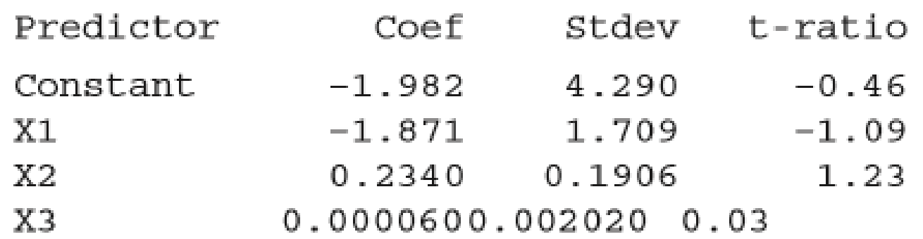
s = 4.189 R-sq = 55.2% R-sq(adj) = 48.8%
Analysis of Variance
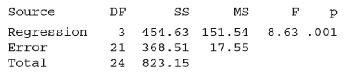
- a. Use information from the Minitab output to test the hypothesis H0: β1 = β2 = β3 = 0.
- b. Using an elimination criterion of −2 ≤ t ratio ≤ 2, should any variable be eliminated? If so, which one?
- c. Minitab output for the regression using only x1 = Sex and x2 = Length is given. Would you recommend keeping both and x2 in the model? Explain.
The regression equation is Y = −2.09 − 1.87X1 + .240X2
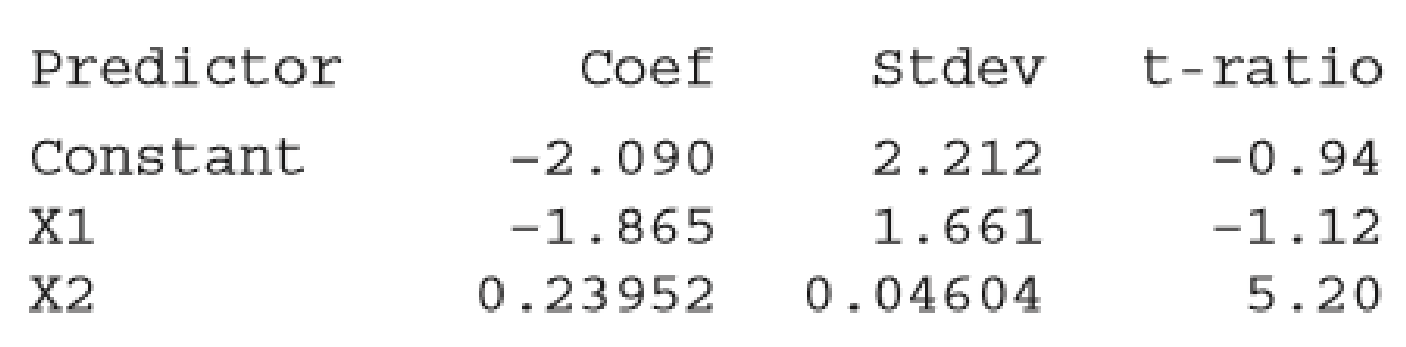
s = 4.093 R-sq = 55.2% R-sq(adj) = 51.2%
- d. After elimination of both x3 and x1, the estimated regression equation is ŷ = −2.61 + 0.231x2. The corresponding values of R2 and se are 0.527 and 4.116, respectively. Interpret these values.
- e. Referring to Part (d), how would you interpret the value of b2 = 0.231? Does it make sense to interpret the value of a as the estimate of average progesterone level when length is zero? Explain.
Want to see the full answer?
Check out a sample textbook solution
Chapter 14 Solutions
Bundle: Introduction to Statistics and Data Analysis, 5th + WebAssign Printed Access Card: Peck/Olsen/Devore. 5th Edition, Single-Term


- Consider the following simple regression model of house prices: house_price = β0 + β1*land_size + u. What could be included in u? Name 2 examples.arrow_forwardGuéguen and Jacob (2012) asked waitresses to wear different colored T-shirts on differentdays for a six-week period and recorded the lips left by male customers. The results show that male customers gave significantly bigger tips to waitresses when they were wearing red. For this study, identify the independent variable and the dependent variable.arrow_forwardAnemia (low healthy blood cells or hemoglobin) has an important role in exercise performance. However, the direct link between rapid changes of hemoglobin and exercise performance is still unknown. A study investigated 18 patients with a blood disorder (beta-thalassemia). Participants in the study performed an exercise test before and the day after receiving a blood transfusion. Data are given in the table. HB = Hemoglobin RER = Respiratory exchange ID Change in HB Obese RER > 1.1 ratio No No 1 -1.4 No -1.5 No Yes No Yes 3 -2 No 4 -2.1 No -1.9 Yes Yes No -1.6 -1.8 -0.8 6 7 No Yes No Yes 8 9. -1 No No -1.2 No Yes 10 11 No No -0.8 -1.5 12 Yes No No Yes 13 14 -1.4 -2.6 -1.7 No No Yes Yes 15 Yes No Yes Yes 16 -2.6 No 17 18 -2.7 -1.5 Noarrow_forward
- Researchers are studying pomegranate’s antioxidant properties to see if it might have any beneficial effects in the treatment of cancer. One such study investigated whether pomegranate fruit extract (PFE) was effective in slowing the growth of prostate cancer tumors. In this study, 24 mice were injected with cancer cells, then the mice were randomly assigned to one of three treatment groups. The data on y = average tumor volume (in mm3) and x = number of days after injection of cancer cells for the mice that received plain drinking water is shown in picture below: a. Find (to three decimal places) zy, and zxzy for the pair (23,580): zy = zxzy = b. Compute Pearson’s sample correlation coefficient for the given data to four decimal places. c. Compute the slope, b, for the least-squares regression line to two decimal places d. Use b to calculate a and write the equation for the least-squares regression line a= y= e. Predict the average tumor volume (y) for a mouse 20 days…arrow_forwardA regression between foot length(response variable in cm) and height (eexplanatory variable in inches) for 33 students resulted in the following regression equation: y^=10,9+0,23X one student in the sample was 73 inches tall with a foot length of 29cm.What is the predicted foot length for A)33cm B)17,57cm C)27,69cm D)29cmarrow_forwardAn article used an estimated regression equation to describe the relationship between y = error percentage for subjects reading a four-digit liquid crystal display and the independent variables x1 = level of backlight, x2 = character subtense, x3 = viewing angle, and x4 = level of ambient light. From a table given in the article, SSRegr = 20.4, SSResid = 21, and n = 30. Calculate the test statistic and calculate P- value. (Round your answer to two decimal places.) F = P- value=arrow_forward
- The table below shows the parameters for four multiple linear regression bridge deterioration models. The full model has age as continuous independent variable, traffic (Average Daily Traffic (ADT)) and bridge design as categorical variables. The bridge design is expressed as codes “H’ or “HS” for a single-unit truck and a tractor pulling a semitrailer respectively. The numeric suffix represents the gross weight in tons for H truck or weight on the first two axle sets of the HS truck. For example, H_10 denotes a truck with a gross work of 10 tons. The table also contains the following model validation indicators: adjusted r-squared, Akaike’s Information Criteria (AIC), Mean Absolute Error (MAE) and Bayesian Information Criteria (BIC). Write the multiple regression equation for each of the four models and comment on the accuracy of prediction of bridge deterioration of each model.arrow_forwardThe table below shows the parameters for four multiple linear regression bridge deterioration models. The full model has age as continuous independent variable, traffic (Average Daily Traffic (ADT)) and bridge design as categorical variables. The bridge design is expressed as codes “H’ or “HS” for a single-unit truck and a tractor pulling a semitrailer respectively. The numeric suffix represents the gross weight in tons for H truck or weight on the first two axle sets of the HS truck. For example, H_10 denotes a truck with a gross work of 10 tons. The table also contains the following model validation indicators: adjusted r-squared, Akaike’s Information Criteria (AIC), Mean Absolute Error (MAE) and Bayesian Information Criteria (BIC). Which model is the best predictor model, give logical justification for your answer. Discuss how these models are utilized in Highway Asset management.arrow_forwardA study of obesity and metabolic syndrome used data collected from 15 students, and included systolic blood pressure (SBP), weight, and BMI. These data are presented in Table 2 (See data 3). Correlations for the three variables are shown in Figure 1. The very large and significant correlation between the variables weight and BMI suggests that including both of these variables in the model is inappropriate because of the high level of redundancy in the information provided by these variables. This makes logical sense since BMI is a function of weight. How to decide which of the variables to retain for constructing the regression model? Table 2 Data from 8 Random Sample of 15 Students Case NO SBP WEIGHT(lbs.) BMI metabolic syndrome 1 126 125 24.41 0 2 129 130 23.77 0 3 126 132 20.07 0 4 123 200 27.12 1 5 124 321 39.07 1 6 125 100 20.9 0 127 138 22.96 0 125 138 24.44 0 123 149 23.33 0 19 180 25.82 0 127 184 26.4 0 126 251 31.87 1 122 197 26.72 1 126 107 20.22 0 125 125 23.62 0 7 8 9 10 11…arrow_forward
- In MANOVA, main effects and interaction are assessed on multiple dependent variables (DVs). True or Falsearrow_forwardA medical student at a community college in city Q wants to study the factors affecting the systolic blood pressure of a person (Y). Generally, the systolic blood pressure depends on the BMI of a person (B) and the age of the person A. She wants to test whether or not the BMI has a significant effect on the systolic blood pressure, keeping the age of the person constant. For her study, she collects a random sample of 150 patients from the city and estimates the following regression function: Y= 15.50 +0.90B + 1.10A. (0.48) (0.35) The test statistic of the study the student wants to conduct (Ho: B, =0 vs. H4: B, #0), keeping other variables constant is. (Round your answer to two decimal places.) At the 5% significance level, the student will v the null hypothesis. Keeping BMI constant, she now wants test whether the age of a person (A) has no significant effect or a positive effect on the person's systolic blood pressure. So, the test statistic associated with the one-sided test the…arrow_forwardCoastal State University is conducting a study regarding the possible relationship between the cumulative grade point average and the annual income of its recent graduates. A random sample of 147 Coastal State graduates from the last five years was selected, and it was found that the least-squares regression equation relating cumulative grade point average (denoted by x, on a 4-point scale) and annual income (denoted by y, in thousands of dollars) was y = 37.79+5.51x. The standard error of the slope of this least-squares regression line was approximately 2.10. Test for a significant linear relationship between grade point average and annual income for the recent graduates of Coastal State by doing a hypothesis test regarding the population slope B1. (Assume that the variable y follows a normal distribution for each value of x and that the other regression assumptions are satisfied.) Use the 0.05 level of significance, and perform a two-tailed test. Then complete the parts below. (If…arrow_forward
 MATLAB: An Introduction with ApplicationsStatisticsISBN:9781119256830Author:Amos GilatPublisher:John Wiley & Sons Inc
 Probability and Statistics for Engineering and th...StatisticsISBN:9781305251809Author:Jay L. DevorePublisher:Cengage Learning
 Statistics for The Behavioral Sciences (MindTap C...StatisticsISBN:9781305504912Author:Frederick J Gravetter, Larry B. WallnauPublisher:Cengage Learning
 Elementary Statistics: Picturing the World (7th E...StatisticsISBN:9780134683416Author:Ron Larson, Betsy FarberPublisher:PEARSON
 The Basic Practice of StatisticsStatisticsISBN:9781319042578Author:David S. Moore, William I. Notz, Michael A. FlignerPublisher:W. H. Freeman
 Introduction to the Practice of StatisticsStatisticsISBN:9781319013387Author:David S. Moore, George P. McCabe, Bruce A. CraigPublisher:W. H. Freeman