
Concept explainers
Videos
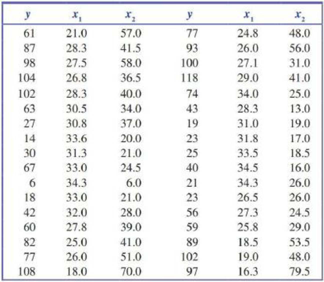
This exercise requires the use of a statistical software package. The cotton aphid poses a threat to cotton crops. The accompanying data on
appeared in the article “Estimation of the Economic Threshold of Infestation for Cotton Aphid” (Mesopotamia Journal of Agriculture [1982]: 71–75). Use the data to find the estimated regression equation and assess the utility of the multiple regression model
Want to see the full answer?
Check out a sample textbook solution
Chapter 14 Solutions
Introduction To Statistics And Data Analysis


- Suppose that a regional express delivery service company wants to estimate the cost of shipping a package (Y) as a function of cargo type, where cargo type includes the following possibilities: fragile, semi-fragile, and durable. Costs for 15 randomly chosen packages of approximately the same weight and same distance shipped, but of different cargo types, are provided in the file P14_16.xlsx. a. Estimate a regression equation using the given sample data, and interpret the estimated regression coefficients. b. According to the estimated regression equation, which cargo type is the most costly to ship? Which cargo type is the least costly to ship? c. How well does the estimated equation fit the given sample data? How might the fit be improved? d. Given the estimated regression equation, predict the cost of shipping a package with semi-fragile cargo.arrow_forwardAnd run a simple linear regression in SPSS to determine if pulse at warm-up (The name of the variable in SPSS is "stage 1" and its label is "pulse at warmup") significantly predicts pulse while running ( The name of the variable in SPSS is "stage 3" and its label is "pulse running"). Use α = .05 Is the regression equation significant? That is, does pulse at warm-up explains (or predicts) a significant amount of variability in pulse while running? Report the F, df (of numerator, and df of the denominator) and p-value.arrow_forwardThe systolic blood pressure dataset (in the third sheet of the spreadsheet linked above) contains the systolic blood pressure and age of 30 randomly selected patients in a medical facility. What is the equation for the least square regression line where the independent or predictor variable is age and the dependent or response variable is systolic blood pressure? Y=__________ X + ______________ Patient 7 is 67 years old and has a systolic blood pressure of 170 mm Hg. What is the residual? __________ mm Hg Is the actual value above, below, or on the line? What is the interpretation of the residual? (difference in actual &predicated bp, difference in age, the amount of systolic changes)arrow_forward
- A sociologist was hired by a large city hospital to investigate the relationship between the number of unauthorized days that employees are absent per year and the distance (miles) between home and work for the employee. A sample of 10 employees was chosen, and the following data were collected. A. Is the estimated regression equation appropriate and adequatearrow_forwardIt is required to use the data given in the table to estimate the parameters of the simple linear regression equation by any of the estimation methods:arrow_forwardIf I want to estimate the regression of a model by using OLS on Eveiws , and I chose the "keep it as general as possible" approach, what tests can I apply through the estimation and inference process to validate the model and the variables?arrow_forward
- The estimated regression equation for a model involving two independent variables and 10 observations follows.arrow_forwardWhich of the multivariate regression parameters listed below would be best interpreted as: the predicted value on the dependent variable when all of the independent variables in the model are equal to zero. a b1 X1 R2arrow_forwardThe linregress() method in scipy module is used to fit a simple linear regression model using “Reaction” (reaction time) as the response variable and “Drinks” as the predictor variable. The output is shown below. What is the correct regression equation based on this output? Is this model statistically significant at 5% level of significance (alpha = 0.05)? Select one. Python script outputs for the linregress method. Slope equals 6.0000, intercept = 3.9999, rvalue = 0.9728, pvalue = 0.0011, stderror = 0.7141. Note: Python output shows many decimal places. All values Question 2 options: Reaction = 6.0000 + 3.9999 Drinks, model is not statistically significant Reaction = 6.0000 + 3.9999 Drinks, model is statistically significant Reaction = 3.9999 + 6.0000 Drinks, model is not statistically significant Reaction = 3.9999 + 6.0000 Drinks, model is statistically significantarrow_forward
- Given a generic data set (x,y) with a linear regression. How do you determine if the y(dependent) will be less/greater than a certain value at a decided value of x?arrow_forwardSuppose the following data were collected from a sample of 15 houses relating selling price to square footage and the architectural style of the house. Use statistical software to find the following regression equation: PRICEi=b0+b1SQFTi+b2COLONIALi+b3RANCHi+ei . Is there enough evidence to support the claim that on average, houses that are ranch style have lower selling prices than houses that are Victorian style at the 0.05 level of significance? If yes, write the regression equation in the spaces provided with answers rounded to two decimal places. Else, select "There is not enough evidence."Selling Price Square Footage Colonial (1 if house is Colonial style, 0 otherwise) Ranch (1 if house is Ranch style, 0 otherwise) Victorian (1 if house is Victorian style, 0 otherwise) 377640 1941 1 0 0 460996 3397 0 1 0 405781 2764 0 0 1 407216 2906 0 0 1 435139 3401 1 0 0 405275 2600 0 0 1 381141 2203 0 1 0 370490 2046 1 0 0 404070 2210 0 0 1 460196 3692 0 1 0 382780 2172 1 0 0 406466 2606 0 1…arrow_forwardA Ross MAP team is currently developing a regression model to explain the travel expense of HR consulting firms in a month (measured in thousands of dollars). So far, the team has identified the number of consultants, the number of clients, the number of air-travel trips, and the number of trips to high-expense cities (e.g., NYC, Boston, San Jose) as potential independent variables. A partial output of the corresponding regression model is in Figure 1. Use the figure to answer question 4to6 4. What is the R2 and adjusted R2 of the model? 5. What is the standard error of the estimates (serror) in thousands of dollars? 6. Based on what you can learn from this table, what is your assessment about the model? For your information, the firm with the lowest travel expense was $47K and the firm with the highest expense was $125K in the sample data.arrow_forward
 College AlgebraAlgebraISBN:9781305115545Author:James Stewart, Lothar Redlin, Saleem WatsonPublisher:Cengage Learning