Introductory Statistics, Books a la Carte Plus NEW MyLab Statistics with Pearson eText -- Access Card Package (10th Edition)
10th Edition
ISBN: 9780134270364
Author: Neil A. Weiss
Publisher: PEARSON
expand_more
expand_more
format_list_bulleted
Concept explainers
Videos
Textbook Question
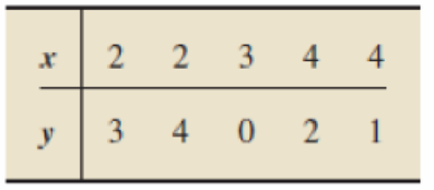
Chapter 14.4, Problem 139E
In Exercises 14.134–14.143, we repeat data from exercises in Section 14.2. For each exercise, determine the linear
- a. Definition 14.8 on page 645.
- b. Formula 14.3 on page 647.
Compare your answers in parts (a) and (b).
14.139
Expert Solution & Answer
Want to see the full answer?
Check out a sample textbook solution
Students have asked these similar questions
Using the data in Table 6–11, calculate a 3-month moving average forecast for month 12.
Q1. The table provided gives data on indexes of output per hour (X) and real compensation per hour (Y) for the business and nonfarm business sectors of the U.S. economy for 1960–2005. The base year of the indexes is 1992 = 100 and the indexes are seasonally adjusted.
a. Plot Y against X for the two sectors separately.
b. What is the economic theory behind the relationship between the two variables? Does the scattergram support the theory?
c. Estimate the OLS regression of Y on X.
Note: on the table ( 1. Output refers to real gross domestic product in the sector. 2. Wages and salaries of employees plus employers’ contributions for social insurance and private benefit plans. 3. Hourly compensation divided by the consumer price index for all urban consumers for recent quarters.)
Thank you!
Exercise 3.12
Chapter 14 Solutions
Introductory Statistics, Books a la Carte Plus NEW MyLab Statistics with Pearson eText -- Access Card Package (10th Edition)
Ch. 14.1 - Regarding linear equations with one independent...Ch. 14.1 - Prob. 2ECh. 14.1 - Consider the linear equation y = b0 + b1x. a....Ch. 14.1 - Prob. 4ECh. 14.1 - In Exercises 14.514.14, we give linear equations....Ch. 14.1 - Prob. 6ECh. 14.1 - In Exercises 14.5-14.14, we give linear equations....Ch. 14.1 - Prob. 8ECh. 14.1 - Prob. 9ECh. 14.1 - In Exercises 14.514.14, we give linear equations....
Ch. 14.1 - Prob. 11ECh. 14.1 - Prob. 12ECh. 14.1 - Prob. 13ECh. 14.1 - Prob. 14ECh. 14.1 - In Exercises 14.1514.22,we identify the...Ch. 14.1 - Prob. 16ECh. 14.1 - Prob. 17ECh. 14.1 - Prob. 18ECh. 14.1 - Prob. 19ECh. 14.1 - Prob. 20ECh. 14.1 - Prob. 21ECh. 14.1 - Prob. 22ECh. 14.1 - Rental-Car Costs. During one month, the Avis...Ch. 14.1 - Air-Conditioning Repairs. Richards Healing and...Ch. 14.1 - Measuring Temperature. The two most commonly used...Ch. 14.1 - A Law of Physics. A ball is thrown straight up in...Ch. 14.1 - Prob. 27ECh. 14.1 - Prob. 28ECh. 14.1 - Prob. 29ECh. 14.1 - Prob. 30ECh. 14.1 - Prob. 31ECh. 14.1 - Road Grade. The grade of a road is defined as the...Ch. 14.1 - Vertical Lines. In this section, we stated that...Ch. 14.2 - Regarding a scatterplot, a. identify one of its...Ch. 14.2 - Regarding the criterion used to decide on the line...Ch. 14.2 - Regarding the line that best fits a set of data...Ch. 14.2 - Regarding the two variables under consideration in...Ch. 14.2 - Using the regression equation to make predictions...Ch. 14.2 - Fill in the blanks. a. In the context of...Ch. 14.2 - For which of the following sets of data points can...Ch. 14.2 - For which of the following sets of data points can...Ch. 14.2 - In each of Exercises 14.4214.45, we have presented...Ch. 14.2 - In each of Exercises 14.4214.45, we have presented...Ch. 14.2 - In each of Exercises 14.4214.45, we have presented...Ch. 14.2 - In each of Exercises 14.4214.45, we have presented...Ch. 14.2 - For a data set consisting of two data points: a....Ch. 14.2 - Prob. 47ECh. 14.2 - In each of Exercises 14.4814.57, a. find the...Ch. 14.2 - In each of Exercises 14.4814.57. a. find the...Ch. 14.2 - In each of Exercises 14.4814.57, a. find the...Ch. 14.2 - In each of Exercises 14.48-14.57, a. find the...Ch. 14.2 - In each of Exercises 14.4814.57, a. find the...Ch. 14.2 - In each of Exercises 14.4814.57, a. find the...Ch. 14.2 - In each of Exercises 14.48-14.57, a. find the...Ch. 14.2 - In each of Exercises 14.4814.57. a. find the...Ch. 14.2 - In each of Exercises 14.4814.57. a. find the...Ch. 14.2 - In each of Exercises 14.4814.57. a. find the...Ch. 14.2 - Prob. 58ECh. 14.2 - In each of Exercises 14.5814.63, a. find the...Ch. 14.2 - In each of Exercises 14.5814.63. a. find the...Ch. 14.2 - In each of Exercises 14.5814.63, a. find the...Ch. 14.2 - In each of Exercises 14.5814.63. a. find the...Ch. 14.2 - In each of Exercises 14.5814.63, a. find the...Ch. 14.2 - Tax Efficiency. In Exercise 14.58, you determined...Ch. 14.2 - Corvette Prices. In Exercise 14.59, you determined...Ch. 14.2 - Anscombes Quartet. In the article Graphs in...Ch. 14.2 - Study Time and Score. The negative relation...Ch. 14.2 - Age and Price of Orions. In Table 14.2, we...Ch. 14.2 - Wasp Mating Systems. In the paper "Mating System...Ch. 14.2 - In Exercises 14.7014.80, use the technology of...Ch. 14.2 - In Exercises 14.7014.80, use the technology of...Ch. 14.2 - In Exercises 14.7014.80, use the technology of...Ch. 14.2 - In Exercises I4.7014.80, use the technology of...Ch. 14.2 - In Exercises 14.7014.80, use the technology of...Ch. 14.2 - In Exercises 14.7014.80, use the technology of...Ch. 14.2 - Prob. 76ECh. 14.2 - Prob. 77ECh. 14.2 - Prob. 78ECh. 14.2 - Prob. 79ECh. 14.2 - In Exercises 14.7014.80, use the technology of...Ch. 14.2 - Prob. 81ECh. 14.2 - Time Series. A collection of observations of a...Ch. 14.3 - In this section, we introduced a descriptive...Ch. 14.3 - A measure of total variation in the observed...Ch. 14.3 - A measure of the amount of variation in the...Ch. 14.3 - A measure of the amount of variation in the...Ch. 14.3 - Prob. 87ECh. 14.3 - In Exercises 14.8814.97, we repeal the data and...Ch. 14.3 - In Exercises14.481497, we repeal the tiara and...Ch. 14.3 - In Exercises 14.8814.97, we repeat the data and...Ch. 14.3 - Prob. 91ECh. 14.3 - Prob. 92ECh. 14.3 - Prob. 93ECh. 14.3 - Prob. 94ECh. 14.3 - Prob. 95ECh. 14.3 - Prob. 96ECh. 14.3 - Prob. 97ECh. 14.3 - Applying the Concepts and Skills For Exercises...Ch. 14.3 - Prob. 99ECh. 14.3 - Prob. 100ECh. 14.3 - Prob. 101ECh. 14.3 - Prob. 102ECh. 14.3 - For Exercises 14.9814.103, a. compute SST, SSR,...Ch. 14.3 - Prob. 104ECh. 14.3 - In Exercises 14.10414.115, use the technology of...Ch. 14.3 - Prob. 106ECh. 14.3 - Prob. 107ECh. 14.3 - Prob. 108ECh. 14.3 - Prob. 109ECh. 14.3 - Prob. 110ECh. 14.3 - Prob. 111ECh. 14.3 - Prob. 112ECh. 14.3 - Prob. 113ECh. 14.3 - In Exercises 14.10414.115, use the technology of...Ch. 14.3 - In Exercises 14.10414.115, use the technology of...Ch. 14.3 - What can you say about SSE, SSR, and the utility...Ch. 14.3 - As we noted, because of the regression identity,...Ch. 14.4 - What is one purpose of the linear correlation...Ch. 14.4 - Prob. 119ECh. 14.4 - The symbol that is used for the linear correlation...Ch. 14.4 - A value of r close to 1 indicates that there is a...Ch. 14.4 - A value of r close to ____ indicates that there is...Ch. 14.4 - A value of r close to ____ indicates that the...Ch. 14.4 - A value of r close to 0 indicates that the...Ch. 14.4 - If y tends to increase linearly as x increases,...Ch. 14.4 - If y lends to decrease linearly as x increases,...Ch. 14.4 - If there is no linear relationship between x and...Ch. 14.4 - In each of Exercises 14.12814.130, determine...Ch. 14.4 - In each of Exercises 14.12814.130, determine...Ch. 14.4 - In each of Exercises 14.12814.130, determine...Ch. 14.4 - Answer true or false to the following statement...Ch. 14.4 - The linear correlation coefficient of a set of...Ch. 14.4 - The coefficient of determination of a set of data...Ch. 14.4 - In Exercises 14.13414.143, we repeat data from...Ch. 14.4 - In Exercises 14.13414.143, we repeat data from...Ch. 14.4 - In Exercises 14.13414.143, we repeat data front...Ch. 14.4 - Prob. 137ECh. 14.4 - In Exercises 14.13414.143, we repeat data from...Ch. 14.4 - In Exercises 14.13414.143, we repeat data from...Ch. 14.4 - In Exercises 14.13414.143, we repeat data from...Ch. 14.4 - In Exercises 14.13414.143, we repeat data from...Ch. 14.4 - In Exercises 14.13414.143, we repeat data from...Ch. 14.4 - In Exercises 14.13414.143, we repeat data from...Ch. 14.4 - In Exercises 14.14414.149, we repeat data from...Ch. 14.4 - In Exercises 14.14414.149, we repeat data from...Ch. 14.4 - In Exercises 14.14414.149, we repeat data from...Ch. 14.4 - Prob. 147ECh. 14.4 - In Exercises 14.14414.149, we repeat data from...Ch. 14.4 - In Exercises 14.14414.149, we repeat data from...Ch. 14.4 - Height and Score. A random sample of 10 students...Ch. 14.4 - Prob. 151ECh. 14.4 - Prob. 152ECh. 14.4 - Prob. 153ECh. 14.4 - Prob. 154ECh. 14.4 - In Exercise 14.154-14.166, use the technology of...Ch. 14.4 - Prob. 156ECh. 14.4 - Prob. 157ECh. 14.4 - Prob. 158ECh. 14.4 - Prob. 159ECh. 14.4 - Prob. 160ECh. 14.4 - Prob. 161ECh. 14.4 - In Exercises 14.154-14.166, use the technology of...Ch. 14.4 - In Exercises 14.15414.166, use the technology of...Ch. 14.4 - Prob. 164ECh. 14.4 - Prob. 165ECh. 14.4 - In Exercises 14.154-14.166, use the technology of...Ch. 14.4 - The coefficient of determination of a set of data...Ch. 14.4 - Country Music Blues. A Knight-Ridder News Service...Ch. 14.4 - Prob. 169ECh. 14.4 - In each of Exercises 14.169 and 14.170, a....Ch. 14 - For a linear equation y = b0 + b1x, identify the ...Ch. 14 - Consider the linear equation y = 4-3x. a. At what...Ch. 14 - In Problems 35, answer true or false to each...Ch. 14 - In Problems 35, answer true or false to each...Ch. 14 - In Problems 35, answer true or false to each...Ch. 14 - Prob. 6RPCh. 14 - In Problems 35, answer true or false to each...Ch. 14 - Prob. 8RPCh. 14 - In each of Problems 911, fill in the blank. 9....Ch. 14 - Prob. 10RPCh. 14 - Prob. 11RPCh. 14 - Prob. 12RPCh. 14 - Prob. 13RPCh. 14 - Prob. 14RPCh. 14 - Prob. 15RPCh. 14 - Prob. 16RPCh. 14 - Prob. 17RPCh. 14 - Prob. 18RPCh. 14 - Prob. 19RPCh. 14 - Equipment Depreciation. A small company has...Ch. 14 - Graduation Rates. Graduation ratethe percentage of...Ch. 14 - Graduation Rates. Refer to Problem 21. a....Ch. 14 - Graduation Rates. Refer to Problem 21. a. Compute...Ch. 14 - Exotic Plants. In the article Effects of Human...Ch. 14 - In Problems 2527, use the technology of your...Ch. 14 - Prob. 26RPCh. 14 - Prob. 27RPCh. 14 - Recall from Chapter 1 (see page 34) that the Focus...Ch. 14 - At the beginning of this chapter, we presented...
Knowledge Booster


Learn more about
Need a deep-dive on the concept behind this application? Look no further. Learn more about this topic, statistics and related others by exploring similar questions and additional content below.Similar questions
- 2.62 For the period 2001–2008, the Bristol-Myers Squibb Company, Inc. reported the following amounts (in billions of dollars) for (1) net sales and (2) advertising and product promotion. The data are also in the file XR02062. Source: Bristol-Myers Squibb Company, Annual Reports, 2005, 2008. Year Net Sales Advertising/Promotion 2001 $16.612 $1.201 2002 16.208 1.143 2003 18.653 1.416 2004 19.380 1.411 2005 19.207 1.476 2006 16.208 1.304 2007 18.193 1.415 2008 20.597 1.550 For these data, construct a line graph that shows both net sales and expenditures for advertising/product promotion over time. Some would suggest that increases in advertising should be accompanied by increases in sales. Does your line graph support this?arrow_forwardQ. Table provided gives data on gross domestic product (GDP) for the United States for the years 1959–2005. a. Plot the GDP data in current and constant (i.e., 2000) dollars against time. b. Letting Y denote GDP and X time (measured chronologically starting with 1 for 1959, 2 for 1960, through 47 for 2005), see if the following model fits the GDP data: Yt = β1 + β2 Xt + ut Estimate this model for both current and constant-dollar GDP. c. How would you interpret β2? d. If there is a difference between β2 estimated for current-dollar GDP and that estimated for constant-dollar GDP, what explains the difference? e. From your results what can you say about the nature of inflation in the United States over the sample period?arrow_forwardRegression and Predictions. Exercises 13–28 use the same data sets as Exercises 13–28 in Section 10-1. In each case, find the regression equation, letting the first variable be the predictor (x) variable. Find the indicated predicted value by following the prediction procedure summarized in Figure 10-5 on page 493. Old Faithful Using the listed duration and interval after times, find the best predicted “interval after” time for an eruption with a duration of 253 seconds. How does it compare to an actual eruption with a duration of 253 seconds and an interval after time of 83 minutes?arrow_forward
- The file P02_26.xlsx lists sales (in millions of dollars) of Dell Computer during the period 1987–1997 (where year 1 corresponds to 1987). Year Sales 1 69 2 159 3 258 4 389 5 546 6 890 7 2014 8 2873 9 3475 10 5296 11 7759 a. Fit a power and an exponential trend curve to these data. Which fits the data better? b. Use your part a answer to predict 1999 sales for Dell. c. Use your part a answer to describe how the sales of Dell have grown from year to year.arrow_forwardNielsen tracks the amount of time that people spend consuming media content across different platforms (digital, audio, television) in the United States. Nielsen has found that traditional television viewing habits vary based on the age of the consumer as an increasing number of people consume media through streaming devices.† The following data represent the weekly traditional TV viewing hours in 2016 for a sample of 14 people aged 18–34 and 12 people aged 35–49. (Round your answers to two decimal places.) Viewers aged 18–34 24.2 21.0 17.8 19.6 23.4 19.1 14.6 27.1 19.2 18.3 22.9 23.4 17.3 20.5 Viewers aged 35–49 24.9 34.9 35.8 31.9 35.4 29.9 30.9 36.7 36.2 33.8 29.5 30.8 (a) Compute the mean and median weekly hours of traditional TV viewed by those aged 18–34.arrow_forwardA researcher is conducting a study to examine the relationship between age and agility. She recruited a sample of 50 participants, ranging in age from 20 – 65 years old, and asked them to perform a series of agility tests. Afterward, participants were given an average agility score, which was then used in a correlation analysis against participant age. The results of the study are as follows [r(50) = -0.97, p < 0.001]. Identify the correct interpretation below. A. There is a non-significant, weak, negative correlation between age and agility, suggest that as age increases, agility decreases B. There is a statistically significant, strong, negative correlation between age and agility, suggesting that as age increases, agility decreases C. There is a non-significant, moderate, positive correlation between age and agility, suggesting that there is no relationship between these two variables D. There is a statistically significant, strong positive correlation between age and…arrow_forward
- In Exercises 1–3, use the data listed below. The values are departure delay times (minutes) for American Airlines flights from New York to Los Angeles. Negative values correspond to flights that departed early. Test for Normality Use the departure delay times for Flight 19 and test for normality using a normal quantile plot.arrow_forward4. The data below represent the number of fatal commercial airline incidents in the United States foreach year from 1998–2011. Find the mode.1 2 3 6 0 2 2 3 2 1 2 1 0 0 5. The table shows the list of average high temperatures in degrees Farenheit for each of the month ofthe year on an island country. Find the mode. Month Jan Feb Mar Apr May Jun Jul Aug Sep Oct Nov Dec 81 82 82 83 85 86 87 87 87 86 84 82 6. Five hundred college graduates were asked how much they donate to their alma mater on an annualbasis. Find the mode of the responses. Responses Frequency$500 or more 45Between 0 to $500 150Nothing 275Refused to answer 30 7. The data shows the number of losses by the team that won the NCAA men’s basketball championshipfor the year…arrow_forwardDATAfile: TelevisionViewing Nielsen tracks the amount of time that people spend consuming media content across different platforms (digital, audio, television) in the United States. Nielsen has found that traditional television viewing habits vary based on the age of the consumer as an increasing number of people consume media through streaming devices.† The following data represent the weekly traditional TV viewing hours in 2016 for a sample of 14 people aged 18–34 and 12 people aged 35–49. (Round your answers to two decimal places.) Viewers aged 18–34 24.2 21.0 17.8 19.6 23.4 19.1 14.6 27.1 19.2 18.3 22.9 23.4 17.3 20.5 Viewers aged 35–49 24.9 34.9 35.8 31.9 35.4 29.9 30.9 36.7 36.2 33.8 29.5 30.8 (a) Compute the mean and median weekly hours of traditional TV viewed by those aged 18–34. mean hrmedian hr (b) Compute the mean and median weekly hours of traditional TV viewed by those aged 35–49. (Round your mean to two decimal places.) mean…arrow_forward
- In 2010, MonsterCollege surveyed 1250 U.S.college students expecting to graduate in the next several years.Respondents were asked the following question:What do you think your starting salary will be at your firstjob after college?The line graph shows the percentage of college students whoanticipated various starting salaries. Use the graph to solveExercises 9–14. What starting salary was anticipated by the greatestpercentage of college students? Estimate the percentage ofstudents who anticipated this salary? What starting salary was anticipated by the least percentageof college students? Estimate the percentage of students whoanticipated this salary? What starting salaries were anticipated by more than 20% ofcollege students? Estimate the percentage of students who anticipated astarting salary of $40 thousand.arrow_forwardA flight travels daily from Pittsburgh to San Antonio. The following list gives the arrival time relative to the scheduled arrival time (in minutes) for a selection of 17 days. (A negative number means that the flight arrived early.) −8, −4, −4, −3, −2, 1, 2, 3, 5, 7, 8, 8, 14, 18, 24, 28, 37 Send data to calculator Frequency 8. 6. 4 2. 5 -10 7 Answer the questions below. 2 0 10 20 30 Arrival time relative to 5:07 (in minutes) 2 (a) For these data, which measures of central tendency take more than one value? Choose all that apply. 1 Mean Median O Mode 40 None of these measuresarrow_forward21–23. Language enrollments. The line graph in Figure 2.28 shows total course enrollments in languages other than English in U.S. institutions of higher education from 1960 to 2009. (Enrollments in ancient Greek and Latin are not included.) Exercises 21 through 23 refer to this figure. 1,800,000 1,629,326 1.522.770 1,600,000 - 1,400,000 - 1347.036 1,200,000- 1,073,097 1,067,217 1,000.000 - 975.7m 963,930 883.222 1.06.603 922,439 960.588 B00,000 - 97.077 877.91 600,000 - 608,749 400.000 - 200,000 - 1960 1965 1968 | 1972 1977 1980 1983 1986 1990 1995 199 2002 2006 2009 1970 1974 Figure 2.28 Crauder, et al., Quantitative Literacy, 3e, © 2019 W. H. Freeman and Company FIGURE 2.28 Enrollments in languages other than English in U.S. institutions of higher education (2009). 21. During which time periods did the enrollments decrease? 22. Calculate the average growth rate per year in enrollments over the two periods 1960–1965 and 2006– 2009. Note that the time periods are not of the same…arrow_forward
arrow_back_ios
SEE MORE QUESTIONS
arrow_forward_ios
Recommended textbooks for you
 MATLAB: An Introduction with ApplicationsStatisticsISBN:9781119256830Author:Amos GilatPublisher:John Wiley & Sons Inc
 Probability and Statistics for Engineering and th...StatisticsISBN:9781305251809Author:Jay L. DevorePublisher:Cengage Learning
 Statistics for The Behavioral Sciences (MindTap C...StatisticsISBN:9781305504912Author:Frederick J Gravetter, Larry B. WallnauPublisher:Cengage Learning
 Elementary Statistics: Picturing the World (7th E...StatisticsISBN:9780134683416Author:Ron Larson, Betsy FarberPublisher:PEARSON
 The Basic Practice of StatisticsStatisticsISBN:9781319042578Author:David S. Moore, William I. Notz, Michael A. FlignerPublisher:W. H. Freeman
 Introduction to the Practice of StatisticsStatisticsISBN:9781319013387Author:David S. Moore, George P. McCabe, Bruce A. CraigPublisher:W. H. Freeman
MATLAB: An Introduction with Applications
Statistics
ISBN:9781119256830
Author:Amos Gilat
Publisher:John Wiley & Sons Inc
Probability and Statistics for Engineering and th...
Statistics
ISBN:9781305251809
Author:Jay L. Devore
Publisher:Cengage Learning
Statistics for The Behavioral Sciences (MindTap C...
Statistics
ISBN:9781305504912
Author:Frederick J Gravetter, Larry B. Wallnau
Publisher:Cengage Learning
Elementary Statistics: Picturing the World (7th E...
Statistics
ISBN:9780134683416
Author:Ron Larson, Betsy Farber
Publisher:PEARSON
The Basic Practice of Statistics
Statistics
ISBN:9781319042578
Author:David S. Moore, William I. Notz, Michael A. Fligner
Publisher:W. H. Freeman
Introduction to the Practice of Statistics
Statistics
ISBN:9781319013387
Author:David S. Moore, George P. McCabe, Bruce A. Craig
Publisher:W. H. Freeman
Correlation Vs Regression: Difference Between them with definition & Comparison Chart; Author: Key Differences;https://www.youtube.com/watch?v=Ou2QGSJVd0U;License: Standard YouTube License, CC-BY
Correlation and Regression: Concepts with Illustrative examples; Author: LEARN & APPLY : Lean and Six Sigma;https://www.youtube.com/watch?v=xTpHD5WLuoA;License: Standard YouTube License, CC-BY