
STATISTICS F/BUS.+ECON.-18WK. MYSTATLAB
13th Edition
ISBN: 9780135901526
Author: MCCLAVE
Publisher: PEARSON
expand_more
expand_more
format_list_bulleted
Concept explainers
Videos
Textbook Question
Chapter 14.8, Problem 14.38LM
The annual price of a finished product (in cents per pound) from 2000 to 2015 is given in the table below. The time variable t begins with t = 1 in 2000 and is incremented by 1 for each additional year
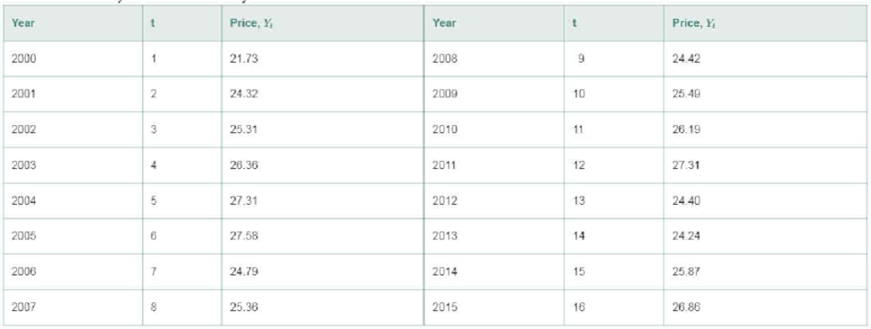
a. Fit the straight-line model, E(Yt) = β0. + β1t, to the data.
b. Give the least squares estimates of the β′s.
c. Use the least squares prediction equation to obtain the forecasts for 2016 and 2017.
d. Find 95% forecast intervals for 2016 and 2017.
Expert Solution & Answer
Want to see the full answer?
Check out a sample textbook solution
Students have asked these similar questions
For the regression model Yi = b0 + eI, derive the least squares estimator.
Compute the least-squares regression equation for the given data set. Round the slope and
y-intercept to at least four decimal places.
2
4
7
6
6
5
3
3
4
2
Consider the following table containing unemployment rates for a 10-year period.
Unemployment Rates
Year
Unemployment Rate (%)
1
5.85.8
2
3.23.2
3
5.55.5
4
8.68.6
5
6.16.1
6
6.86.8
7
7.57.5
8
5.25.2
9
11.111.1
10
7.47.4
Step 1 of 2 :
Given the model
Estimated Unemployment Rate=β0+β1(Year)+εi,Estimated Unemployment Rate=�0+�1(Year)+��,
write the estimated regression equation using the least squares estimates for β0�0 and β1�1. Round your answers to two decimal places.
Chapter 14 Solutions
STATISTICS F/BUS.+ECON.-18WK. MYSTATLAB
Ch. 14.1 - Explain in words how to construct a simple index.Ch. 14.1 - Explain in words how to calculate the following...Ch. 14.1 - Explain in words the difference between Laspeyres...Ch. 14.1 - The table below gives the prices for three...Ch. 14.1 - Refer to Exercise 14.4. The next table gives the...Ch. 14.1 - Annual median family income. The table below lists...Ch. 14.1 - Annual U.S. craft beer production. While overall...Ch. 14.1 - Quarterly single-family housing starts. The...Ch. 14.1 - Spot price of natural gas. The table shown in the...Ch. 14.1 - Employment in farm and nonfarm categories....
Ch. 14.1 - GOP personal consumption expenditures. The gross...Ch. 14.1 - GDP personal consumption expenditures (contd)....Ch. 14.1 - Weekly earnings for workers. The table in the next...Ch. 14.1 - Production and price of metals. The level or price...Ch. 14.2 - Describe the effect of selecting an exponential...Ch. 14.2 - A monthly time series is shown in the table to the...Ch. 14.2 - Annual U.S. craft beer production. Refer to the...Ch. 14.2 - Foreign fish production. Overfishing and pollution...Ch. 14.2 - Yearly price of gold. The price of gold is used by...Ch. 14.2 - Personal consumption in transportation. There has...Ch. 14.2 - OPEC crude oil imports. The data in the table...Ch. 14.2 - SP 500 Stock Index. Standard Poors 500 Composite...Ch. 14.5 - How does the choice of the smoothing constant w...Ch. 14.5 - Refer to Exercise 14.4 (p. 14-9). The table with...Ch. 14.5 - Annual U.S. craft beer production. Refer to...Ch. 14.5 - Quarterly single-family housing starts. Refer to...Ch. 14.5 - Consumer Price Index. The CPI measures the...Ch. 14.5 - OPEC crude oil imports. Refer to the annual OPEC...Ch. 14.5 - SP 500 Stock Index. Refer to the quarterly...Ch. 14.5 - SP 500 Stock Index (contd). Refer to Exercise...Ch. 14.5 - Monthly gold prices. The fluctuation of gold...Ch. 14.6 - Annual U.S. craft beer production. Refer to the...Ch. 14.6 - Annual U.S. craft beer production (contd). Refer...Ch. 14.6 - SP 500 Stock Index. Refer to your exponential...Ch. 14.6 - SP 500 Stock Index (contd). Refer to your Holt...Ch. 14.6 - Monthly gold prices. Refer to the monthly gold...Ch. 14.6 - US school enrollments. The next table reports...Ch. 14.8 - The annual price of a finished product (in cents...Ch. 14.8 - Retail sales in Quarters 14 over a 10-year period...Ch. 14.8 - What advantage do regression forecasts have over...Ch. 14.8 - Mortgage interest rates. The level at which...Ch. 14.8 - Price of natural gas. Refer to Exercise 14.9 (p....Ch. 14.8 - A gasoline tax on carbon emissions. In an effort...Ch. 14.8 - Predicting presidential elections. Researchers at...Ch. 14.8 - Life insurance policies in force. The table below...Ch. 14.8 - Graphing calculator sales. The next table presents...Ch. 14.8 - Prob. 14.47ACICh. 14.9 - Define autocorrelation. Explain why it is...Ch. 14.9 - For each case, indicate the decision regarding the...Ch. 14.9 - What do the following Durbin-Watson statistics...Ch. 14.9 - Company donations to charity. Refer to the Journal...Ch. 14.9 - Forecasting monthly car and truck sales. Forecasts...Ch. 14.9 - Predicting presidential elections. Refer to the...Ch. 14.9 - Mortgage interest rates. Refer to the data on...Ch. 14.9 - Price of natural gas. Refer to the annual data on...Ch. 14.9 - Life insurance policies in force. Refer to the...Ch. 14.9 - Modeling the deposit share of a retail bank....Ch. 14 - Insured Social Security workers. Workers insured...Ch. 14 - Insured Social Security workers (contd). Refer to...Ch. 14 - Retail prices of food items. In 1990, the average...Ch. 14 - Demand for emergency room services. With the...Ch. 14 - Mortgage interest rates. Refer to the annual...Ch. 14 - Price of Abbott Labs stock. The yearly closing...Ch. 14 - Price o f Abbott Labs stock (contd). Refer to...Ch. 14 - Prob. 14.65ACICh. 14 - Prob. 14.66ACICh. 14 - Quarterly GOP values (contd). Refer to Exercise...Ch. 14 - Prob. 14.68ACICh. 14 - Prob. 14.69ACICh. 14 - Prob. 14.70ACICh. 14 - IBM stock prices. Refer to Example 14.1 (p. 14-5)...Ch. 14 - Prob. 14.72ACI
Knowledge Booster


Learn more about
Need a deep-dive on the concept behind this application? Look no further. Learn more about this topic, statistics and related others by exploring similar questions and additional content below.Similar questions
- The following fictitious table shows kryptonite price, in dollar per gram, t years after 2006. t= Years since 2006 0 1 2 3 4 5 6 7 8 9 10 K= Price 56 51 50 55 58 52 45 43 44 48 51 Make a quartic model of these data. Round the regression parameters to two decimal places.arrow_forwardOlympic Pole Vault The graph in Figure 7 indicates that in recent years the winning Olympic men’s pole vault height has fallen below the value predicted by the regression line in Example 2. This might have occurred because when the pole vault was a new event there was much room for improvement in vaulters’ performances, whereas now even the best training can produce only incremental advances. Let’s see whether concentrating on more recent results gives a better predictor of future records. (a) Use the data in Table 2 (page 176) to complete the table of winning pole vault heights shown in the margin. (Note that we are using x=0 to correspond to the year 1972, where this restricted data set begins.) (b) Find the regression line for the data in part ‚(a). (c) Plot the data and the regression line on the same axes. Does the regression line seem to provide a good model for the data? (d) What does the regression line predict as the winning pole vault height for the 2012 Olympics? Compare this predicted value to the actual 2012 winning height of 5.97 m, as described on page 177. Has this new regression line provided a better prediction than the line in Example 2?arrow_forward(a) Find the equation of the least-squares line for the data. (Round all numerical values to two decimal places.) y= ?arrow_forward
- The following Minitab display gives information regarding the relationship between the body weight of a child (in kilograms) and the metabolic rate of the child (in 100 kcal/ 24 hr). Predictor Coef SE Coef T PConstant 0.8570 0.4148 2.06 0.84Weight 0.38243 0.02978 13.52 0.000 S = 0.517508 R-Sq = 97.4% (a) Write out the least-squares equation. y^= ______ + _____x (b) For each 1 kilogram increase in weight, how much does the metabolic rate of a child increase? (Use 5 decimal places.)arrow_forwardThe following table lists the birth weights (in pounds), x, and the lengths (in inches), y, for a set of newborn babies at a local hospital. Birth Weights and Lengths Birth Weight (in Pounds), x 4 8 10 4 12 7 10 10 6 5 Length (in Inches), y 16 20 18 17 21 19 19 20 18 15 Step 1 of 2 : Find an equation of the least-squares regression line. Round your answer to three decimal places, if necessary. instructions for if/how to do this on the TI84 would be greatly appreciated :)arrow_forwardThe following Minitab display gives information regarding the relationship between the body weight of a child (in kilograms) and the metabolic rate of the child (in 100 kcal/ 24 hr). Predictor Coef SE Coef T P Constant 0.8651 0.4148 2.06 0.84 Weight 0.40619 0.02978 13.52 0.000 S = 0.517508 R-Sq = 97.0% (a) Write out the least-squares equation. y = + x (b) For each 1 kilogram increase in weight, how much does the metabolic rate of a child increase? (Use 5 decimal places.)(c) What is the value of the correlation coefficient r? (Use 3 decimal places.)arrow_forward
arrow_back_ios
arrow_forward_ios
Recommended textbooks for you
 Linear Algebra: A Modern IntroductionAlgebraISBN:9781285463247Author:David PoolePublisher:Cengage Learning
 Functions and Change: A Modeling Approach to Coll...AlgebraISBN:9781337111348Author:Bruce Crauder, Benny Evans, Alan NoellPublisher:Cengage Learning
 Algebra & Trigonometry with Analytic GeometryAlgebraISBN:9781133382119Author:SwokowskiPublisher:Cengage
 College AlgebraAlgebraISBN:9781305115545Author:James Stewart, Lothar Redlin, Saleem WatsonPublisher:Cengage Learning
Linear Algebra: A Modern Introduction
Algebra
ISBN:9781285463247
Author:David Poole
Publisher:Cengage Learning
Functions and Change: A Modeling Approach to Coll...
Algebra
ISBN:9781337111348
Author:Bruce Crauder, Benny Evans, Alan Noell
Publisher:Cengage Learning
Algebra & Trigonometry with Analytic Geometry
Algebra
ISBN:9781133382119
Author:Swokowski
Publisher:Cengage
College Algebra
Algebra
ISBN:9781305115545
Author:James Stewart, Lothar Redlin, Saleem Watson
Publisher:Cengage Learning
Correlation Vs Regression: Difference Between them with definition & Comparison Chart; Author: Key Differences;https://www.youtube.com/watch?v=Ou2QGSJVd0U;License: Standard YouTube License, CC-BY
Correlation and Regression: Concepts with Illustrative examples; Author: LEARN & APPLY : Lean and Six Sigma;https://www.youtube.com/watch?v=xTpHD5WLuoA;License: Standard YouTube License, CC-BY