
Videos
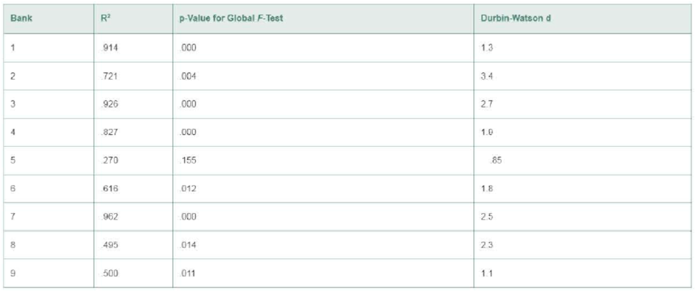
Modeling the deposit share of a retail bank. Exploratory research published in the Journal of Professional Services Marketing (Vol. 5, 1990) examined the relationship between deposit share of a retail bank and several marketing variables. Quarterly deposit share data were collected for 5 consecutive years for each of nine retail banking institutions. The model analyzed took the following form:
E(Yt) = β0 + β1Pt−1 + β2St−1 + β3Dt−1
where Yt = deposit share of a bank In quarter t (t = 1, 2, ... , 20), Pt−1 = expenditures on promotion-related activities in quarter t – 1, St−1 = expenditures on service- related activities in quarter t − 1, and Dt−1 = expenditures on distribution-related activities in quarter t – 1. A separate model was fit for each bank with the results shown in the table.
a. Interpret the values of R2 for each bank.
b. Test the overall adequacy of the model for each bank using α = .01.
c. Conduct the Durbin-Watson d-test for
Want to see the full answer?
Check out a sample textbook solution
Chapter 14 Solutions
STATISTICS F/BUS.+ECON.-18WK. MYSTATLAB


- In a typical multiple linear regression model where x1 and x2 are non-random regressors, the expected value of the response variable y given x1 and x2 is denoted by E(y | 2,, X2). Build a multiple linear regression model for E (y | *,, *2) such that the value of E(y | x1, X2) may change as the value of x2 changes but the change in the value of E(y | X1, X2) may differ in the value of x1 . How can such a potential difference be tested and estimated statistically?arrow_forwardThe accompanying data file contains 40 observations on the response variable y along with the predictor variables x and d. Consider two linear regression models where Model 1 uses the variables x and d and Model 2 extends the model by including the interaction variable xd. Use the holdout method to compare the predictability of the models using the first 30 observations for training and the remaining 10 observations for validation. y x d 70 11 1 102 19 1 76 12 1 83 14 1 61 17 0 62 13 0 67 20 0 98 16 1 84 11 1 101 15 1 51 16 0 108 16 1 32 13 0 71 15 1 101 17 1 90 15 1 112 19 1 88 13 1 110 18 1 95 17 1 44 14 0 51 19 0 112 17 1 113 17 1 52 13 0 61 10 1 100 16 1 78 14 1 90 16 1 57 16 0 59 15 0 53 15 0 119 19 1 109 18 1 68 11 0 104 19 1 45 18 0 67 17 0 65 15 0 74 14 1 1. Use the training set to estimate Models 1 and 2. Note: Negative values should be indicated by a minus sign. Round your answers to 2…arrow_forwardSecond-Hand Smoke: Data Set 12 “Passive and Active Smoke” in Appendix B includes cotinine levels measured in a group of nonsmokers exposed to tobacco smoke (n = 40, Mean = 60.58 ng>mL, s = 138.08 ng>mL) and a group of nonsmokers not exposed to tobacco smoke (n = 40, Mean = 16.35 ng>mL, s = 62.53 ng>mL). Cotinine is a metabolite of nicotine, meaning that when nicotine is absorbed by the body, cotinine is produced. Use a 0.05 significance level to test the claim that nonsmokers exposed to tobacco smoke have a higher mean cotinine level than nonsmokers not exposed to tobacco smoke. Construct the confidence interval appropriate for the hypothesis test in part a. What do you conclude about the effects of second-hand smoke?arrow_forward
- Explain the Gauss–Markov Conditions for Multiple Regression?arrow_forwardAn article in Biotechnology Progress (2001, Vol. 17, pp. 366-368) reported on an experiment to investigate and optimize nisin extraction in aqueous two-phase systems. The nisin recovery was the dependent variable (y). The two regressor variables were concentration (%) of PEG 4000 (x1) and concentration (%) of Na2SO4 (x2) : Form the Multiple Regression Model using Matrices. Y = ___ + ___ X1 + ___ X2arrow_forwardWhat are homoskedasticity and heteroskedasticity in multiple linear regression? How would you check for heteroskedasticity in a multiple linear regression model?arrow_forward
- The monthly premium quoted by an insurance company for a critical illness policy was collected from a sample of 6 adult male smokers at different age. The data for the sample are shown: Age 28 25 50 39 47 31 Premium ($) 75 40 175 125 250 105 Using Age to predict premium, the Linear Regression equation is given by: ŷ =6.556X−112 and r2=0.813y^=6.556X−112 and r2=0.813 a. Identify the independent and Dependent variables. Dependent: Age Premium Independent: Age Premium b. Determine the slope. Slope = Slope = Round to 3 decimal places c. Determine |r||r| . |r|=|r|= Round to 3 decimal places d. Interpret rr : and e. Determine critical r value at 5% significance level and determine if there is a significant linear correlation exists. |r| critical=|r| critical= Round to 3 decimal places Linear Correlation:Linear Correlation: Significant Not Significant f. Predict the monthly premium for a 40 years old adult male smoker.…arrow_forwardThe accompanying data file contains 40 observations on the response variable y along with the predictor variables x1 and x2. Use the holdout method to compare the predictability of the linear model with the exponential model using the first 30 observations for training and the remaining 10 observations for validation. y x1 x2 533.86 20 30 104.84 15 20 64.89 20 23 159.61 16 21 43.06 13 16 4.27 13 13 736.56 15 30 64.89 20 23 10.64 20 22 76.90 18 20 4.89 11 13 80.90 11 16 224.17 12 19 45.75 16 25 8.13 17 17 319.97 13 30 48.61 19 25 564.67 12 27 111.87 11 25 152.39 13 24 13.34 18 14 28.80 15 22 37.56 13 15 105.62 17 26 44.05 18 21 451.65 17 28 10.34 18 21 32.70 12 13 19.21 14 12 14.02 15 16 2.45 16 12 2.48 20 15 50.34 17 21 29.31 17 20 33.75 16 12 196.28 17 29 943.12 13 30 7.25 10 12 89.73 15 25 32.91 12 18 1. Use the training set to estimate Models 1 and 2. Note: Negative values should be indicated by a…arrow_forwardA study was conducted to assess the impact of nutrient enrichment on zooplankton densities in A & B Islands. An ecologist sampled populations of zooplankton in these two locations and observed the nutrient enrichment level was higher in A island when compared with the level in B island. It is predicted the zooplankton densities in A island will be greater than those found in B island.arrow_forward
- In a simple linear regression model, the correlation coefficient between x and y is 0.8. What can you say about the strength and direction of the relationship between x and y?arrow_forwardThe table shows a part of an output of a linear regression model predicting the average fare on different flight routes. Data Table Regression Table Coefficient Constant 95.80976147 COUPON −9.61654124 DISTANCE 0.080733811 PAX −0.000167343 What is the difference in prediction of the following two routes? Route A that is 3,000 miles, with COUPON=1.5 and PAX=6,000 Route B that is 3,000 miles, with COUPON=1.2 and PAX=6,000.arrow_forwardA strain of genetically engineered cotton, known as Bt cotton, is resistant to certain insects, which results in larger yields of cotton. Farmers in northern China have increased the number of acres planted in Bt cotton. Because Bt cotton is resistant to certain pests, farmers have also reduced their use of insecticide. Scientists in China were interested in the long‑term effects of Bt cotton cultivation and decreased insecticide use on insect populations that are not affected by Bt cotton. One such insect is the mirid bug. Scientists measured the number of mirid bugs per 100 plants and the proportion of Bt cotton planted at 38 locations in northern China for the 12‑year period from 1997–2008. The scientists reported this regression analysis: number of mirid bugs per 100 plants=0.54+6.81× Bt cotton planting proportion ?2=0.90, ?<0.0001 What does the slope b=6.81 say about the relation between Bt cotton planting proportion and number of mirid bugs per 100 plants? - Scientists…arrow_forward
 MATLAB: An Introduction with ApplicationsStatisticsISBN:9781119256830Author:Amos GilatPublisher:John Wiley & Sons Inc
 Probability and Statistics for Engineering and th...StatisticsISBN:9781305251809Author:Jay L. DevorePublisher:Cengage Learning
 Statistics for The Behavioral Sciences (MindTap C...StatisticsISBN:9781305504912Author:Frederick J Gravetter, Larry B. WallnauPublisher:Cengage Learning
 Elementary Statistics: Picturing the World (7th E...StatisticsISBN:9780134683416Author:Ron Larson, Betsy FarberPublisher:PEARSON
 The Basic Practice of StatisticsStatisticsISBN:9781319042578Author:David S. Moore, William I. Notz, Michael A. FlignerPublisher:W. H. Freeman
 Introduction to the Practice of StatisticsStatisticsISBN:9781319013387Author:David S. Moore, George P. McCabe, Bruce A. CraigPublisher:W. H. Freeman