
Introduction to Statistics and Data Analysis
5th Edition
ISBN: 9781305750999
Author: Peck Olson Devore
Publisher: CENGAGE C
expand_more
expand_more
format_list_bulleted
Concept explainers
Videos
Textbook Question
Chapter 15.2, Problem 20E
The accompanying data resulted from a flammability study in which specimens of five different fabrics were tested to determine burn times.
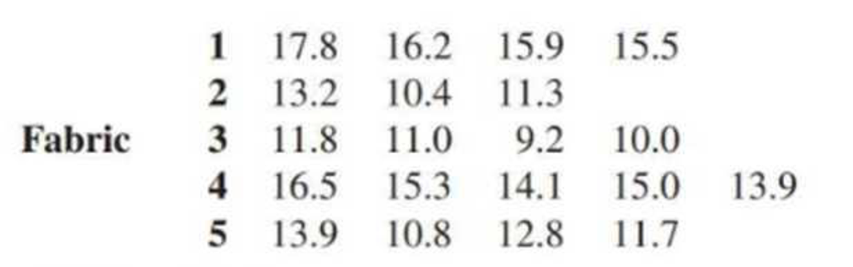
MSTr = 23.67
MSE = 1.39
F = 17.08
P-value = 0.000
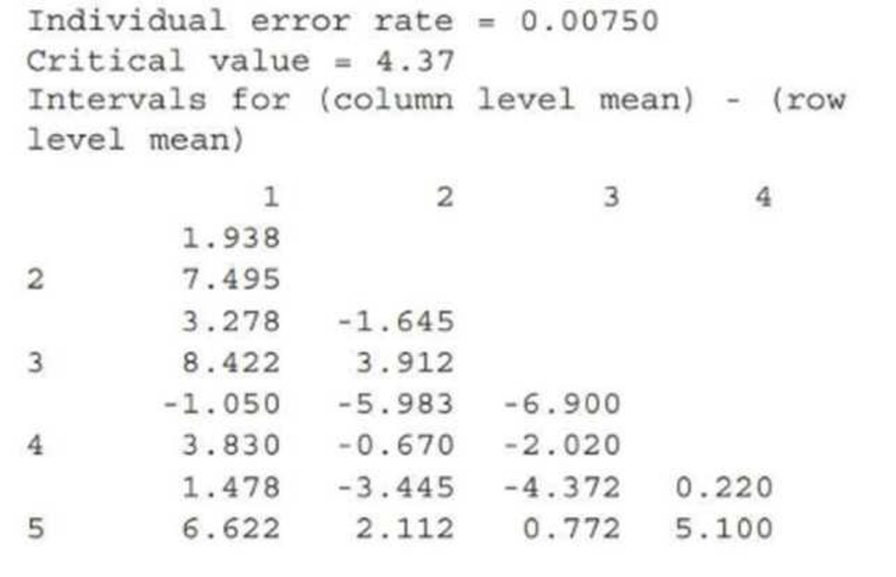
The accompanying output gives the T-K intervals as calculated by Minitab. Identify significant differences and give the underscoring pattern.
Expert Solution & Answer

Trending nowThis is a popular solution!

Students have asked these similar questions
Glaucoma is a leading cause of blindness in the United States, N. Ehlers measured the difference in corneal thickness (in microns) between the two eyes of eight patients. Each patient had one eye that had glaucoma and one eye that was normal. The difference was measured as the corneal thickness of normal eye – corneal thickness of eye with Glaucoma. Corneal thickness is important because it can mask an accurate reading of eye pressure.
Use ? = .05
H0: μd=0
H1: μd≠0
T statistic: t = 1.053, P value = 0.327
Degrees of Freedom
n-1 = 8-1= 7
critical value
2.3646
If t is less than 2.3646, or greater than 2.3646, reject the null hypothesis
Level of significance:
α=0.05
question:
what a type 1 error and type 2 error would mean. Is it possible that we could have committed a type 2 error in conducting the test
Glaucoma is a leading cause of blindness in the United States, N. Ehlers measured the difference in corneal thickness (in microns) between the two eyes of eight patients. Each patient had one eye that had glaucoma and one eye that was normal. The difference was measured as the corneal thickness of normal eye – corneal thickness of eye with Glaucoma. Corneal thickness is important because it can mask an accurate reading of eye pressure. Use ? = .05.
Q) If a participant has the same corneal thickness in their normal eye as the eye with Glaucoma, what would be the value for difference: measured as the corneal thickness of normal eye – corneal thickness of eye with Glaucoma.
Glaucoma is a leading cause of blindness in the United States, N. Ehlers measured the difference in corneal thickness (in microns) between the two eyes of eight patients. Each patient had one eye that had glaucoma and one eye that was normal. The difference was measured as the corneal thickness of normal eye – corneal thickness of eye with Glaucoma. Corneal thickness is important because it can mask an accurate reading of eye pressure. Use ? = .05.
Q)Conduct a hypothesis test to determine if there is sufficient evidence to conclude that corneal thickness is different in normal eyes compared to eyes with glaucoma? Write up your results using the 8 steps.
Chapter 15 Solutions
Introduction to Statistics and Data Analysis
Ch. 15.1 - Give as much information as you can about the...Ch. 15.1 - Prob. 2ECh. 15.1 - Employees of a state university system can choose...Ch. 15.1 - The accompanying summary statistics for a measure...Ch. 15.1 - The authors of the paper Age and Violent Content...Ch. 15.1 - The paper referenced in the previous exercise also...Ch. 15.1 - The Paper Womens and Mens Eating Behavior...Ch. 15.1 - Can use of an online plagiarism-detection system...Ch. 15.1 - The experiment described in Example 15.4 also gave...Ch. 15.1 - Prob. 10E
Ch. 15.1 - Prob. 11ECh. 15.1 - Prob. 12ECh. 15.1 - In an experiment to investigate the performance of...Ch. 15.2 - Leaf surface area is an important variable in...Ch. 15.2 - Prob. 15ECh. 15.2 - Prob. 16ECh. 15.2 - Prob. 17ECh. 15.2 - The paper referenced in Exercise 15.5 described an...Ch. 15.2 - Prob. 19ECh. 15.2 - The accompanying data resulted from a flammability...Ch. 15.2 - Do lizards play a role in spreading plant seeds?...Ch. 15.2 - Samples of six different brands of diet or...Ch. 15.3 - A particular county employs three assessors who...Ch. 15.3 - The accompanying display is a partially completed...Ch. 15.3 - With the use of biofuels increasing, investigators...Ch. 15.3 - Prob. 26ECh. 15.3 - Prob. 27ECh. 15.3 - Prob. 28ECh. 15.4 - Prob. 29ECh. 15.4 - The paper Feedback Enhances the Positive Effects...Ch. 15.4 - The following graphs appear in the paper Which...Ch. 15.4 - The behavior of undergraduate students when...Ch. 15.4 - Prob. 33ECh. 15.4 - The following partially completed ANOVA table...Ch. 15.4 - Prob. 35ECh. 15.4 - Prob. 36ECh. 15.4 - Prob. 37ECh. 15 - Suppose that a random sample or size n = 5 was...Ch. 15 - Parents are frequently concerned when their child...Ch. 15 - Prob. 40CRCh. 15 - Consider the accompanying data on plant growth...Ch. 15 - Prob. 42CRCh. 15 - Prob. 43CRCh. 15 - Prob. 44CRCh. 15 - Prob. 45CRCh. 15 - Prob. 46CRCh. 15 - Prob. 47CRCh. 15 - Prob. 48CRCh. 15 - Prob. 49CR
Knowledge Booster


Learn more about
Need a deep-dive on the concept behind this application? Look no further. Learn more about this topic, statistics and related others by exploring similar questions and additional content below.Similar questions
- Glaucoma is a leading cause of blindness in the United States, N. Ehlers measured the difference in corneal thickness (in microns) between the two eyes of eight patients. Each patient had one eye that had glaucoma and one eye that was normal. The difference was measured as the corneal thickness of normal eye – corneal thickness of eye with Glaucoma. Corneal thickness is important because it can mask an accurate reading of eye pressure. Use ? = .05. Hypothesis: H0: μd=0Ha: μd≠0 Using output Test statistics : t=0.134P value=0.897 Degrees of freedom (df): df=7 Level of significance: α=0.05 Decision: P value > 0.05 thus we fails to reject null hypothesis. Question a)Write a report summarizing your findings. When writing the report consider that medical staff estimate that a difference of 4.5 microns or more could impact on their ability to interpret eye pressure correctly. b) Define for the hypothesis stated in part b) what a type 1 error and type 2 error would mean. Is it possible…arrow_forwardRefer to the accompanying data display that results from a sample of airport data speeds in Mbps. Complete parts (a) through (c) below. Tinterval (13.046,22.15) x=17.598 Sx=16.01712719 n=50arrow_forwarddont uplode any image in answer answer must be typed,arrow_forward
- The average concentration of cadmium (Cd) in tea leaves sample is 68.0(±1.5) ppm Cd. Calculate .8 * the coefficient of variation (CV) for sample is 2.2 O 0.11 O 0.012 O 3.4 O 0.012 Oarrow_forwardCalculate the missing values, labelled (A) - (D), in this R output, in alphabetical order as labelled in the output.arrow_forwardThe following data are from an experiment on carnations. The explanatory variable is the amount of inorganic bromine (micrograms per milliliter) in a plot of standard size. The response variable is the average number of flowers per carnation plant for the 30 plants grown in the plot. Find the change in number of flowers per plant given an increase in 1 µg per mL of inorganic bromine. Amount of bromine Average no. of flowers Select one: O a. -0.216 O b. 0.216 O c. O d. -3.81 4.04 3 3.2 4 2.9 6 3.7 7 2.2 8 1.8 10 2.3 12 1.7 15 16 0.8 0.3arrow_forward
- A photoconductor film is manufactured at a nominal thickness of 25 mils. The product engineer wishes to increase the mean speed of the film, and believes that this can be achieved by reducing the thickness of the film to 20 mils. Eight samples of each film thickness are manufactured in a pilot production process, and the film speed (in microjoules per square inch) is measured. For the 25-mil film, the sample data result is = 1.15 and 81 = 0.11, while for the 20-mil film, the data yield 2 = 1.06 and 82 = 0.09. Note that an increase in film speed vould lower the value of the observation in microjoules per square inch. (a) Do the data support the claim that reducing the film thickness increases the mean speed of the film? Use a = 0.10 and assume that the two population variances are equal and the underlying population of film speed is normally distributed. What is the P-value for this test? Round your answer to three decimal places (e.g. 98.765). The data the claim that reducing the film…arrow_forwardOcean currents are important in studies of climate change, as well as ecology studies of dispersal of plankton. Drift bottles are used to study ocean currents in the Pacific near Hawaii, the Solomon Islands, New Guinea, and other islands. Let x represent the number of days to recovery of a drift bottle after release and y represent the distance from point of release to point of recovery in km/100. The following data are representative of one study using drift bottles to study ocean currents. Σx = 476, Σy = 87.1, Σx2 = 62,290, Σy2 = 2046.87, Σxy = 11121.3,and r ≈ 0.94367. x days 72 76 32 91 205y km/100 14.7 19.6 5.3 11.7 35.8 a) Use a 1% level of significance to test the claim ? > 0.(Use 2 decimal places.)t =critical t= b) Find the predicted distance (km/100) when a drift bottle has been floating for 60 days. (Use 2 decimal places.)________ km/100 c) Find a 90% confidence interval for your prediction of part (d). (Use 1 decimal place.)lower limit = _____…arrow_forward1.56 Longleaf pine trees. The Wade Tract in Thomas County, Georgia, is an old-growth forest of longleaf pine trees (Pinus palustris) that has survived in a relatively undisturbed state since before the settlement of the area by Europeans. A study collected data on 584 of these trees. One of the variables measured was the diameter at breast height (DBH). This is the diameter of the tree at 4.5 feet, and the units are centimeters (cm). Only trees with DBH greater than 1.5 cm were sampled. Here are the diameters of a random sample of 40 of these trees: PINES 27 10.5 13.3 26.0 18.3 52.2 9.2 26.1 17.6 40.5 31.8 47.2 11.4 2.7 69.3 44.4 16.9 35.7 5.4 44.2 2.2 4.3 7.8 38.1 2.2 11.4 51.5 4.9 39.7 32.6 51.8 43.6 2.3 44.6 31.5 40.3 22.3 43.3 37.5 29.1 27.9 (a) Find the five-number summary for these data. (b) Make a boxplot. (c) Make a histogram. (d) Write a short summary of the major features of this distribution. Do you prefer the boxplot or the histogram for these data?arrow_forward
- A photoconductor film is manufactured at a nominal thickness of 25 mils. The product engineer wishes to increase the mean speed of the film and believes that this can be achieved by reducing the thickness of the film to 20 mils. Eight samples of each film thickness are manufactured in a pilot production process, and the film speed (in microjoules per square inch) is measured. For the 25-mil film, the sample data result is.x₁ = 1.15 and S₁ = 0.11, while for the 20-mil film, the data yield 2 = 1.06 and s2 = 0.09. Note that an increase in film speed would lower the value of the observation in microjoules per square inch. Do the data support the claim that reducing the film thickness increases the mean speed of the film? Use a = 0.10 and assume that the two population variances are equal and the underlying population of film speed is normally distributed. The appropriate decision for the test is to reject the null hypothesis True Falsearrow_forwardFind the five-number summary for the data summarized by the box plotsarrow_forwardAnswer the blanks in red. For the test procedure and p value use image 2arrow_forward
arrow_back_ios
SEE MORE QUESTIONS
arrow_forward_ios
Recommended textbooks for you
 College Algebra (MindTap Course List)AlgebraISBN:9781305652231Author:R. David Gustafson, Jeff HughesPublisher:Cengage Learning
 Glencoe Algebra 1, Student Edition, 9780079039897...AlgebraISBN:9780079039897Author:CarterPublisher:McGraw Hill
College Algebra (MindTap Course List)
Algebra
ISBN:9781305652231
Author:R. David Gustafson, Jeff Hughes
Publisher:Cengage Learning
Glencoe Algebra 1, Student Edition, 9780079039897...
Algebra
ISBN:9780079039897
Author:Carter
Publisher:McGraw Hill
Probability & Statistics (28 of 62) Basic Definitions and Symbols Summarized; Author: Michel van Biezen;https://www.youtube.com/watch?v=21V9WBJLAL8;License: Standard YouTube License, CC-BY
Introduction to Probability, Basic Overview - Sample Space, & Tree Diagrams; Author: The Organic Chemistry Tutor;https://www.youtube.com/watch?v=SkidyDQuupA;License: Standard YouTube License, CC-BY