Chapter 17, Problem 1CP

Forecasting Food and Beverage Sales

The Vintage Restaurant, on Captiva Island near Fort Myers, Florida, is owned and operated by Karen Payne. The restaurant just completed its third year of operation. Since opening her restaurant, Karen has sought to establish a reputation for the Vintage as a high-quality dining establishment that specializes in fresh seafood. Through the efforts of Karen and her staff, her restaurant has become one of the best and fastest growing restaurants on the island.

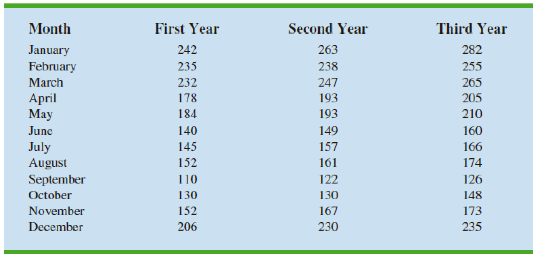
To better plan for future growth of the restaurant, Karen needs to develop a system that will enable her to forecast food and beverage sales by month for up to one year in advance. Table 17.25 shows the value of food and beverage sales ($1000s) for the first three years of operation.

Managerial Report

Perform an analysis of the sales data for the Vintage Restaurant. Prepare a report for Karen that summarizes your findings, forecasts, and recommendations. Include the following:

1. 1. A time series plot. Comment on the underlying pattern in the time series.
2. 2. An analysis of the seasonality of the data. Indicate the seasonal indexes for each month, and comment on the high and low seasonal sales months. Do the seasonal indexes make intuitive sense? Discuss.

   TABLE 17.25 Food and beverage sales for the vintage restaurant ($1000s)

1. 3. Deseasonalize the time series. Does there appear to be any trend in the deseasonalized time series?
2. 4. Using the time series decomposition method, forecast sales for January through December of the fourth year.
3. 5. Using the dummy variable regression approach, forecast sales for January through December of the fourth year.
4. 6. Provide summary tables of your calculations and any graphs in the appendix of your report.

   Assume that January sales for the fourth year turn out to be $295,000. What was your forecast error? If this error is large, Karen may be puzzled about the difference between your forecast and the actual sales value. What can you do to resolve her uncertainty in the forecasting procedure?

To determine

Construct a time series plot and explain the type of pattern.

Answer to Problem 1CP

The time series plot is given below:

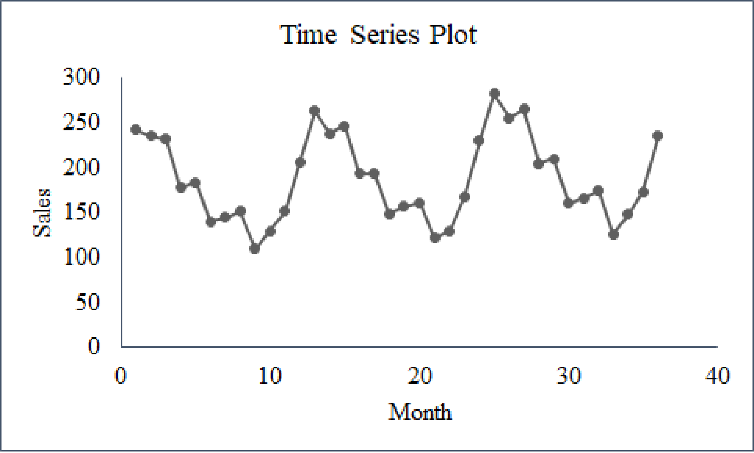
The pattern that appears in the graph is linear in trend with a seasonal pattern.

Explanation of Solution

Calculation:

It is given that Person KP started Restaurant V. Restaurant V is one of the best and fastest growing restaurants on the island. Person KP needs to develop a system that will forecast the food and beverage sales by month for up to one year in advance.

Software procedure:

Step-by-step software procedure to draw the time series plot using EXCEL:

• Open an EXCEL file.
• In column A, enter the data of Month and in column B, enter the data of Sales.
• Select the data that are to be displayed.
• Click on the Insert Tab > select Scatter icon.
• Choose a Scatter with Straight Lines and Markers.
• Click on the chart > select Layout from the Chart Tools.
• Select Chart Title > Above Chart and enter Time Series Plot.
• Select Axis Title > Primary Horizontal Axis Title > Title Below Axis.
• Enter Month in the dialog box.
• Select Axis Title > Primary Vertical Axis Title > Rotated Title.
• Enter Sales in the dialog box.

From the output, the time series plot represents the seasonality of the data. From the three years of the data, it is observed that the month of September has the lowest sales and the month of January has the highest sales every year.

Thus, the pattern that appears in the graph is linear in trend with a seasonal pattern.

To determine

Calculate the seasonal indexes.

Find the high and low seasonal indexes and check whether the seasonal indexes are reasonable or not.

Answer to Problem 1CP

The monthly seasonal indexes are tabulated below:

Month	Seasonal Index
1	1.44
2	1.30
3	1.34
4	1.04
5	1.05
6	0.80
7	0.83
8	0.85
9	0.63
10	0.70
11	0.85
12	1.16

Explanation of Solution

Calculation:

The formula for moving the average forecast of order k is as follows:

$\begin{array}{c}{F}_{t+1}=\frac{{\displaystyle \sum \left(\text{most recent }k\text{data values}\right)}}{k}\\ =\frac{Y_t+Y_{t-1}+\mathrm{...}+Y_{t-k+1}}{k}\end{array}$

$\begin{array}{c}{F}_{t+1}=\text{forecast of the times series of period }t+1\\ Y_t=\text{Actual value of the time series in period }t\end{array}$

For the first moving average:

$\begin{array}{c}\text{Moving average}=\frac{\left(\begin{array}{l}242+235+232+178+184+140+\\ 145+152+110+130+152+206\end{array}\right)}{12}\\ =\frac{2,106}{12}\\ =175.5\end{array}$

For the second moving average:

$\begin{array}{c}\text{Moving average}=\frac{\left(\begin{array}{l}235+232+178+184+140+145+\\ 152+110+130+152+206+263\end{array}\right)}{12}\\ =\frac{2,127}{12}\\ =177.25\end{array}$

For the first centered moving average:

$\begin{array}{c}\text{Centered moving average}=\frac{175.5+177.25}{2}\\ =\frac{352.75}{2}\\ =176.375\end{array}$

Similarly, the remaining moving averages and centered moving averages are obtained as follows:

Month	Sales	Moving Average	Centered Moving Average	$\begin{array}{l}\text{Seasonal Irregular value}\\ \text{=}\frac{\text{Sales}}{\text{Centered MA}}\end{array}$
1	242		–	–
2	235		–	–
3	232		–	–
4	178		–	–
5	184		–	–
6	140		–	–
		175.500
7	145		176.375	0.822
		177.250
8	152		177.375	0.857
		177.500
9	110		178.125	0.618
		178.750
10	130		179.375	0.725
		180.000
11	152		180.375	0.843
		180.750
12	206		181.125	1.137
		181.500
13	263		182.000	1.445
		182.500
14	238		182.875	1.301
		183.250
15	247		183.750	1.344
		184.250
16	193		184.250	1.047
		184.250
17	193		184.875	1.044
		185.500
18	149		186.500	0.799
		187.500
19	157		188.292	0.834
		189.083
20	161		189.792	0.848
		190.500
21	122		191.250	0.638
		192.000
22	130		192.500	0.675
		193.000
23	167		193.708	0.862
		194.417
24	230		194.875	1.180
		195.333
25	282		195.708	1.441
		196.083
26	255		196.625	1.297
		197.167
27	265		197.333	1.343
		197.500
28	205		198.250	1.034
		199.000
29	210		199.250	1.054
		199.500
30	160		199.708	0.801
		199.917
31	166		–	–
32	174		–	–
33	126		–	–
34	148		–	–
35	173		–	–
36	235		–	–

Use the above table to calculate the following:

Months	Seasonal Irregular Values		Seasonal Index
1	1.445	1.441	$\frac{1.445+1.441}{2}=1.44$
2	1.301	1.297	$\frac{1.301+1.297}{2}=1.30$
3	1.344	1.343	$\frac{1.344+1.343}{2}=1.34$
4	1.047	1.034	$\frac{1.047+1.034}{2}=1.04$
5	1.044	1.054	$\frac{1.044+1.054}{2}=1.05$
6	0.799	0.801	$\frac{0.799+0.801}{2}=0.80$
7	0.822	0.834	$\frac{0.822+0.834}{2}=0.83$
8	0.857	0.848	$\frac{0.857+0.848}{2}=0.85$
9	0.618	0.638	$\frac{0.618+0.638}{2}=0.63$
10	0.725	0.675	$\frac{0.725+0.675}{2}=0.70$
11	0.843	0.862	$\frac{0.843+0.862}{2}=0.85$
12	1.137	1.180	$\frac{1.137+1.180}{2}=1.16$

To determine

Compute the deseasonalized time-series.

Check whether the deseasonalized data appear to be of any trend.

Answer to Problem 1CP

Deseasonalized expenses are given below:

Month (Year 1)	Deseasonalized Readings	Month (Year 2)	Deseasonalized Readings	Month (Year 3)	Deseasonalized Readings
1	168.06	1	182.64	1	195.83
2	180.77	2	183.08	2	196.15
3	173.13	3	184.33	3	197.76
4	171.15	4	185.58	4	197.12
5	175.24	5	183.81	5	200.00
6	175.00	6	186.25	6	200.00
7	174.70	7	189.16	7	200.00
8	178.82	8	189.41	8	204.71
9	174.60	9	193.65	9	200.00
10	185.71	10	185.71	10	211.43
11	178.82	11	196.47	11	203.53
12	177.59	12	198.28	12	202.59

The linear trend equation is $\underset{\_}{Y_t=169.50+1.02t}$.

Explanation of Solution

Calculation:

Deseasonalized data are obtained below:

Month	Sales	Adjusted Seasonal Index	$\begin{array}{l}\text{Deseasonalized Sales}\\ =\frac{\text{Time series value}}{\begin{array}{c}\text{Adjusted SI}\end{array}}\end{array}$
1	242	1.44	168.06
2	235	1.30	180.77
3	232	1.34	173.13
4	178	1.04	171.15
5	184	1.05	175.24
6	140	0.80	175.00
7	145	0.83	174.70
8	152	0.85	178.82
9	110	0.63	174.60
10	130	0.70	185.71
11	152	0.85	178.82
12	206	1.16	177.59
13	263	1.44	182.64
14	238	1.30	183.08
15	247	1.34	184.33
16	193	1.04	185.58
17	193	1.05	183.81
18	149	0.80	186.25
19	157	0.83	189.16
20	161	0.85	189.41
21	122	0.63	193.65
22	130	0.70	185.71
23	167	0.85	196.47
24	230	1.16	198.28
25	282	1.44	195.83
26	255	1.30	196.15
27	265	1.34	197.76
28	205	1.04	197.12
29	210	1.05	200.00
30	160	0.80	200.00
31	166	0.83	200.00
32	174	0.85	204.71
33	126	0.63	200.00
34	148	0.70	211.43
35	173	0.85	203.53
36	235	1.16	202.59

Trend:

Software procedure:

Step-by-step software procedure to find the linear trend equation using EXCEL:

• Open an EXCEL file.
• In column A, enter the data of Month and in column B, enter the data of Deseasonalized Sales.
• Select the data that are to be displayed.
• Click on the Insert Tab > select Scatter icon.
• Choose a Scatter with Straight Lines and Markers.
• Click on the chart > select Layout from the Chart Tools.
• Select Chart Title > Above Chart and enter Time Series Plot.
• Select Axis Title > Primary Horizontal Axis Title > Title Below Axis.
• Enter Month in the dialog box.
• Select Axis Title > Primary Vertical Axis Title > Rotated Title.
• Enter Deseasonalized Sales in the dialog box.
• Right Click at any point in the time series plot and select Add Trendline.
• Select Linear under TrendLine Options.
• Choose Display Equation on Chart.

Output obtained using EXCEL is given below:

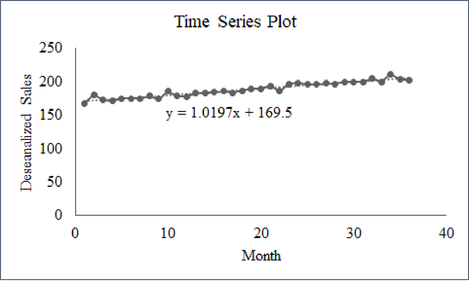
From the output, the linear trend equation is $\underset{\_}{Y_t=169.50+1.0197t}$.

To determine

Compute the adjusted deseasonalized trend forecasts for 12 months of the fourth year.

Answer to Problem 1CP

The adjusted forecast is tabulated below:

Month	Adjusted Forecast
1	298.41
2	27072
3	280.42
4	218.70
5	221.87
6	169.86
7	177.08
8	182.21
9	135.70
10	151.48
11	184.81
12	253.40

Explanation of Solution

Calculation:

The linear trend equation using Part (3) is as follows:

$Y_t=169.50+1.0197t$

The periods for fourth year are 37 to 48.

For the period 37:

$\begin{array}{c}\text{Forecast for month January}=169.50+1.0197\left(37\right)\\ =169.50+37.729\\ \approx 207.228\end{array}$

Similarly, the remaining forecasts for year 4 are obtained as follows:

Period	Year 4	Forecast
37	January	207.229
38	February	208.249
39	March	209.268
40	April	210.288
41	May	211.308
42	June	212.327
43	July	213.347
44	August	214.367
45	September	215.387
46	October	216.406
47	November	217.426
48	December	218.446

Use the seasonal indexes to adjust the forecasts developed in Part (3).

The adjusted forecast is obtained as follows:

$\text{Adjusted forecast for January}=\text{Forecast}\times \text{Seasonal Index}$

For January:

$\begin{array}{c}\text{Adjusted forecast for January}=\text{Forecast for January }\times \text{Seasonal Index for January}\\ \text{=207}\text{.229}\times \text{1}\text{.44}\\ \text{=298}\text{.41}\end{array}$

Year 4	Period	Forecast	Seasonal Index	Adjusted Forecast
January	37	207.229	1.44	298.410
February	38	208.249	1.30	270.724
March	39	209.268	1.34	280.419
April	40	210.288	1.04	218.700
May	41	211.308	1.05	221.873
June	42	212.327	0.80	169.862
July	43	213.347	0.83	177.078
August	44	214.367	0.85	182.212
September	45	215.387	0.63	135.694
October	46	216.406	0.70	151.484
November	47	217.426	0.85	184.812
December	48	218.446	1.16	253.397

To determine

Estimate the forecast sales for January through December of the fourth year using dummy variable.

Answer to Problem 1CP

The forecast sales are tabulated below:

Month	Forecast Sales
1	262.7
2	243
3	248.3
4	192.3
5	196
6	150
7	156.3
8	162.7
9	120
10	136.3
11	164.3
12	224

Explanation of Solution

Calculation:

The regression equation is given below:

$\widehat{Y_t}=b_0+b_1\text{ Month1}+b_2\text{ Month2+}\mathrm{...}+b_{12}\text{ Month12}$

Here

$\begin{array}{c}{Y}_t=\text{Estimate or forecast value in period t}\\ \text{Month 1}=\{\begin{array}{l}1\text{ ; if the time period corresponds to Month1}\\ 0\text{ ; otherwise}\end{array}\end{array}$

…

$\text{Month 12}=\{\begin{array}{l}1\text{ ; if the time period corresponds to Month12}\\ 0\text{ ; otherwise}\end{array}$

Software procedure:

Step-by-step procedure to obtain the estimated regression equation using EXCEL:

• In EXCEL sheet, enter January, February, March, April, May, June, July, September, October, November, Time period and Sales in different columns.
  • In Data, select Data Analysis and choose Regression.
  • In Input Y Range, select S.
• In Input X Range, select January, February, March, April, May, June, July, September, October, November.
  • Select Labels.
  • Click OK.

Output obtained using EXCEL is given below:

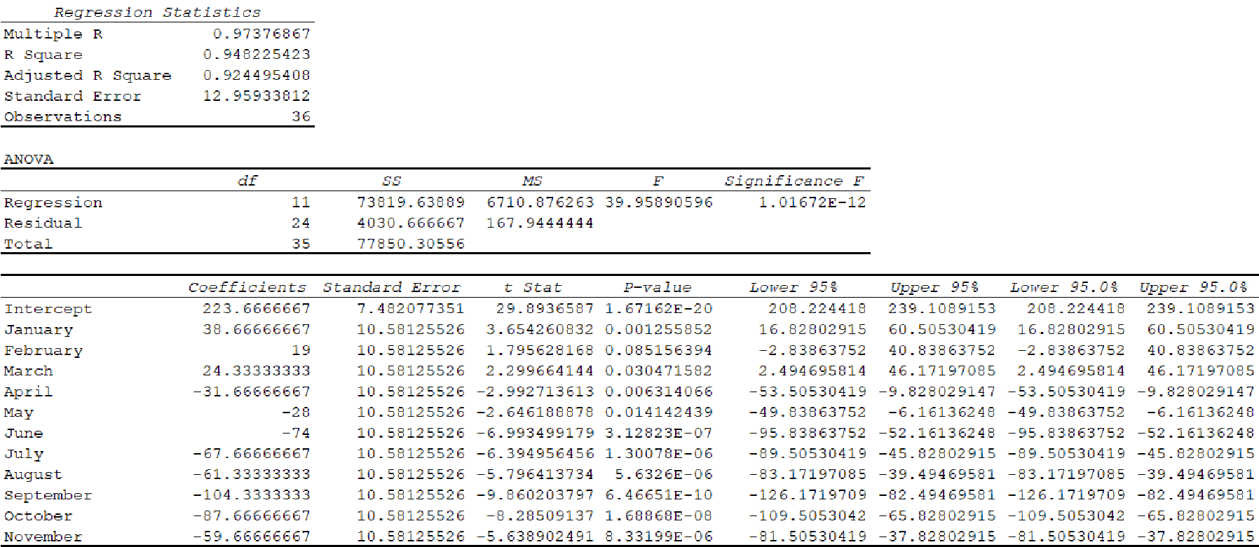
From the results, the regression equation is given below:

$\begin{array}{c}\text{Sales}=224+38.7\text{January}+19.0\text{ February}+24.3\text{ March}-31.7\text{April}\\ -28.0\text{May}-74.0\text{ June }-67.7\text{july}-61.3\text{August}-104\text{September}\\ -87.7\text{October}-59.7\text{November}\end{array}$

The next year monthly forecasts are as follows:

$\begin{array}{c}\text{January forecast = }224+38.7\left(1\right)+19.0\left(0\right)+24.3\left(0\right)-31.7\left(0\right)-28.0\left(0\right)\\ -74.0\left(0\right)-67.7\left(0\right)-61.3\left(0\right)-104\left(0\right)-87.7\left(0\right)-59.7\left(0\right)\\ =224+38.7\\ =262.7\end{array}$

$\begin{array}{c}\text{February forecast = }224+38.7\left(0\right)+19.0\left(1\right)+24.3\left(0\right)-31.7\left(0\right)-28.0\left(0\right)\\ -74.0\left(0\right)-67.7\left(0\right)-61.3\left(0\right)-104\left(0\right)-87.7\left(0\right)-59.7\left(0\right)\\ =224+19.0\\ =243\end{array}$

$\begin{array}{c}\text{March forecast = }224+38.7\left(0\right)+19.0\left(0\right)+24.3\left(1\right)-31.7\left(0\right)-28.0\left(0\right)\\ -74.0\left(0\right)-67.7\left(0\right)-61.3\left(0\right)-104\left(0\right)-87.7\left(0\right)-59.7\left(0\right)\\ =224+24.3\\ =248.3\end{array}$

$\begin{array}{c}\text{April forecast = }224+38.7\left(0\right)+19.0\left(0\right)+24.3\left(0\right)-31.7\left(1\right)-28.0\left(0\right)\\ -74.0\left(0\right)-67.7\left(0\right)-61.3\left(0\right)-104\left(0\right)-87.7\left(0\right)-59.7\left(0\right)\\ =224-31.7\\ =192.3\end{array}$

$\begin{array}{c}\text{May forecast = }224+38.7\left(0\right)+19.0\left(0\right)+24.3\left(0\right)-31.7\left(0\right)-28.0\left(1\right)\\ -74.0\left(0\right)-67.7\left(0\right)-61.3\left(0\right)-104\left(0\right)-87.7\left(0\right)-59.7\left(0\right)\\ =224-28\\ =196\end{array}$

$\begin{array}{c}\text{June forecast = }224+38.7\left(0\right)+19.0\left(0\right)+24.3\left(0\right)-31.7\left(0\right)-28.0\left(0\right)\\ -74.0\left(1\right)-67.7\left(0\right)-61.3\left(0\right)-104\left(0\right)-87.7\left(0\right)-59.7\left(0\right)\\ =224-74\\ =150\end{array}$

$\begin{array}{c}\text{July forecast = }224+38.7\left(0\right)+19.0\left(0\right)+24.3\left(0\right)-31.7\left(0\right)-28.0\left(0\right)\\ -74.0\left(0\right)-67.7\left(1\right)-61.3\left(0\right)-104\left(0\right)-87.7\left(0\right)-59.7\left(0\right)\\ =224-67.7\\ =156.3\end{array}$

$\begin{array}{c}\text{August forecast = }224+38.7\left(0\right)+19.0\left(0\right)+24.3\left(0\right)-31.7\left(0\right)-28.0\left(0\right)\\ -74.0\left(0\right)-67.7\left(0\right)-61.3\left(1\right)-104\left(0\right)-87.7\left(0\right)-59.7\left(0\right)\\ =224-61.3\\ =162.7\end{array}$

$\begin{array}{c}\text{September forecast = }224+38.7\left(0\right)+19.0\left(0\right)+24.3\left(0\right)-31.7\left(0\right)-28.0\left(0\right)\\ -74.0\left(0\right)-67.7\left(0\right)-61.3\left(0\right)-104\left(1\right)-87.7\left(0\right)-59.7\left(0\right)\\ =224-104\\ =120\end{array}$

$\begin{array}{c}\text{October forecast = }224+38.7\left(0\right)+19.0\left(0\right)+24.3\left(0\right)-31.7\left(0\right)-28.0\left(0\right)\\ -74.0\left(0\right)-67.7\left(0\right)-61.3\left(0\right)-104\left(0\right)-87.7\left(1\right)-59.7\left(0\right)\\ =224-87.7\\ =136.3\end{array}$

$\begin{array}{c}\text{November forecast = }224+38.7\left(0\right)+19.0\left(0\right)+24.3\left(0\right)-31.7\left(0\right)-28.0\left(0\right)\\ -74.0\left(0\right)-67.7\left(0\right)-61.3\left(0\right)-104\left(0\right)-87.7\left(0\right)-59.7\left(1\right)\\ =224-59.7\\ =164.3\end{array}$

$\begin{array}{c}\text{December forecast = }224+38.7\left(0\right)+19.0\left(0\right)+24.3\left(0\right)-31.7\left(0\right)-28.0\left(0\right)\\ -74.0\left(0\right)-67.7\left(0\right)-61.3\left(0\right)-104\left(0\right)-87.7\left(0\right)-59.7\left(0\right)\\ =224-0\\ =224\end{array}$

To determine

Give summary tables.

Find the forecast error between the forecast sales and the actual sales.

Explain the solution for the uncertainty in the forecasting procedure.

Explanation of Solution

Calculation:

The summary table of the data is given below:

Month	Seasonal Index	Forecast Sales By deseasonalize data	Forecast Sales By dummy variable
1	1.44	298.410	262.7
2	1.30	270.724	243
3	1.34	280.419	248.3
4	1.04	218.700	192.3
5	1.05	221.873	196
6	0.80	169.862	150
7	0.83	177.078	156.3
8	0.85	182.212	162.7
9	0.63	135.694	120
10	0.70	151.484	136.3
11	0.85	184.812	164.3
12	1.16	253.397	224

It is assumed that the January sales for the fourth year is $295,000.

The forecast January sales using deseasonalized data is $298,410.

The forecast error is calculated as follows:

$\begin{array}{c}\text{Forecast error}=295,000-298,410\\ =-3,410\end{array}$

The forecast value is overpredicted and the difference is –$3,410.

The error is very small, while the sales are of large amount.

The uncertainty in the forecast procedure can be resolved using the monthly forecast.