Concept explainers
Videos
a.
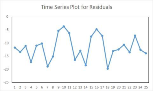
The given plot of residuals in the order in which the data are presented.
a.
Answer to Problem 16E
The plot for the ordered residuals is as follows:
Explanation of Solution
Step-by-step procedure to obtain the regression using EXCEL:
- Enter the data for Commissions, Calls, and Driven in EXCEL sheet.
- Go to Data Menu.
- Click on Data Analysis.
- Select Regression and click on OK.
- Select the column of Commissions under Input Y
Range . - Select the column of Calls and Driven under Input X Range.
- Click on OK.
Output for the Regression obtained using Excel is as follows:
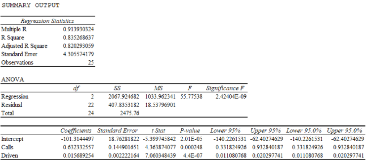
From the Excel output, the regression equation is
Residual:
Formula for residual is
| Commissions | ||
| 22 | 33.67 | −11.67 |
| 13 | 26.36 | −13.36 |
| 33 | 44.02 | −11.02 |
| 38 | 55.16 | −17.16 |
| 23 | 33.92 | −10.92 |
| 47 | 57.12 | −10.12 |
| 29 | 47.9 | −18.9 |
| 38 | 53.09 | −15.09 |
| 41 | 46.24 | −5.24 |
| 32 | 35.6 | −3.6 |
| 20 | 26.15 | −6.15 |
| 13 | 29.37 | −16.37 |
| 47 | 59.92 | −12.92 |
| 38 | 56.46 | −18.46 |
| 44 | 51.46 | −7.46 |
| 29 | 33.73 | −4.73 |
| 38 | 45.22 | −7.22 |
| 37 | 56.73 | −19.73 |
| 14 | 26.95 | −12.95 |
| 34 | 46.36 | −12.36 |
| 25 | 35.64 | −10.64 |
| 27 | 40.5 | −13.5 |
| 25 | 32.11 | −7.11 |
| 43 | 55.46 | −12.46 |
| 34 | 47.87 | −13.87 |
Step-by-step procedure to obtain the plot for Residuals using EXCEL:
- Enter the data for Residuals in Excel sheet.
- Select the column of Residuals.
- Go to Insert Menu.
- Select line chart.
Thus, the plot for the ordered residuals is obtained.
b.
Test the autocorrelation at the 0.01 significance level.
b.
Answer to Problem 16E
There is a positive autocorrelation among the residuals at the 0.01 significance level.
Explanation of Solution
The null and alternative hypotheses are given below:
H0: There is no autocorrelation among the residuals.
H1: There is a positive residual autocorrelation.
Test Statistic:
The Durbin–Watson statistic for testing the hypothesis is as follows:
| y | Lagged Residual, | ||||
| 22 | 33.67 | –11.67 | 136.189 | ||
| 13 | 26.36 | –13.36 | –11.67 | 2.8561 | 178.49 |
| 33 | 44.02 | –11.02 | –13.36 | 5.4756 | 121.44 |
| 38 | 55.16 | –17.16 | –11.02 | 37.6996 | 294.466 |
| 23 | 33.92 | –10.92 | –17.16 | 38.9376 | 119.246 |
| 47 | 57.12 | –10.12 | –10.92 | 0.64 | 102.414 |
| 29 | 47.9 | –18.9 | –10.12 | 77.0884 | 357.21 |
| 38 | 53.09 | –15.09 | –18.9 | 14.5161 | 227.708 |
| 41 | 46.24 | –5.24 | –15.09 | 97.0225 | 27.4576 |
| 32 | 35.6 | –3.6 | –5.24 | 2.6896 | 12.96 |
| 20 | 26.15 | –6.15 | –3.6 | 6.5025 | 37.8225 |
| 13 | 29.37 | –16.37 | –6.15 | 104.448 | 267.977 |
| 47 | 59.92 | –12.92 | –16.37 | 11.9025 | 166.926 |
| 38 | 56.46 | –18.46 | –12.92 | 30.6916 | 340.772 |
| 44 | 51.46 | –7.46 | –18.46 | 121 | 55.6516 |
| 29 | 33.73 | –4.73 | –7.46 | 7.4529 | 22.3729 |
| 38 | 45.22 | –7.22 | –4.73 | 6.2001 | 52.1284 |
| 37 | 56.73 | –19.73 | –7.22 | 156.5 | 389.273 |
| 14 | 26.95 | –12.95 | –19.73 | 45.9684 | 167.703 |
| 34 | 46.36 | –12.36 | –12.95 | 0.3481 | 152.77 |
| 25 | 35.64 | –10.64 | –12.36 | 2.9584 | 113.21 |
| 27 | 40.5 | –13.5 | –10.64 | 8.1796 | 182.25 |
| 25 | 32.11 | –7.11 | –13.5 | 40.8321 | 50.5521 |
| 43 | 55.46 | –12.46 | –7.11 | 28.6225 | 155.252 |
| 34 | 47.87 | –13.87 | –12.46 | 1.9881 | 192.377 |
The test statistic is as follows:
Thus, the Durbin–Watson statistic is 0.22.
Critical value:
From the given information table, there are two independent variables. That is,
The level of significance is 0.01 and the sample size is 25.
From Table Appendix B.9C: Critical values for the Durbin–Watson d Statistic (α=.01), for
Rejection Rule:
- If
- If
- If
Conclusion:
The value of d is 0.22 that is less than 0.98.
That is,
From the rejection rule, reject the null hypothesis.
It can be concluded that there is a positive autocorrelation among the residuals.
Want to see more full solutions like this?
Chapter 18 Solutions
Statistical Techniques in Business and Economics, 16th Edition


 Big Ideas Math A Bridge To Success Algebra 1: Stu...AlgebraISBN:9781680331141Author:HOUGHTON MIFFLIN HARCOURTPublisher:Houghton Mifflin Harcourt
 Glencoe Algebra 1, Student Edition, 9780079039897...AlgebraISBN:9780079039897Author:CarterPublisher:McGraw Hill