
Calculus: Special Edition: Chapters 1-5 (w/ WebAssign)
6th Edition
ISBN: 9781524908102
Author: SMITH KARL J, STRAUSS MONTY J, TODA MAGDALENA DANIELE
Publisher: Kendall Hunt Publishing
expand_more
expand_more
format_list_bulleted
Concept explainers
Videos
Question
Chapter 2, Problem 86SP
(a)
To determine
To graph : Below data points:
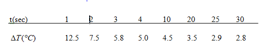
To calculate:Temperature difference
(b)
To determine
To graph : Below data points:
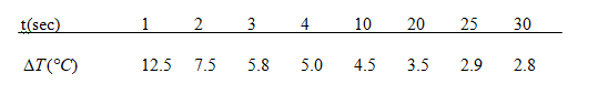
To calculate: Exposure time t, when temperature difference i.e
Expert Solution & Answer
Want to see the full answer?
Check out a sample textbook solution
Students have asked these similar questions
Emissions of sulfur dioxide by industry set off chemical changes in the atmosphere that result in "acid rain".
The acidity of liquids is measured by pH on a scale of 00 to 14.14. Distilled water has pH 7.0,7.0, and lower pH values indicate acidity. Normal rain is somewhat acidic, so "acid rain" is sometimes defined as rainfall with a pH below 5.0.5.0.
The pH of rain at one location varies among rainy days according to a Normal distribution with mean 5.43 and standard deviations 0.54.
What proportion of rainy days have rainfall with pH below 5.0?5.0?
Emissions of sulfur dioxide by industry set off chemical changes in the atmosphere that result in "acid rain". The acidity of liquids is measured by pH on a scale of 00 to 14.14. Distilled water has pH 7.0,7.0, and lower pH values indicate acidity. Normal rain is somewhat acidic, so acid rain is sometimes defined as rainfall with a pH below 5.0.5.0. The pH of rain at one location varies among rainy days according to a Normal distribution with mean 5.435.43 and standard deviation 0.54.deviation 0.54.
What proportion of rainy days have rainfall with pH below 5.0?5.0?
Engineers concerned about a tower's stability have done extensive studies of its increasing tilt. Measurements of the lean of the tower over time provide much useful information. The
following table gives measurements for the years 1975 to 1987. The variable "lean" represents the difference between where a point on the tower would be if the tower were straight and
where it actually is. The data are coded as tenths of a millimeter in excess of 2.9 meters, so that the 1975 lean, which was 2.9647 meters, appears in the table as 647. Only the last two
digits of the year were entered into the computer.
80
83
86
75 76 77 78
647 649 660 672
79
81 82
84 85
678 693 701 703 717 722 729
747
(a) Plot the data. Consider whether or not the trend in lean over time appears to be linear. (Do this on paper. Your instructor may ask you to turn in this graph.)
Year
Lean
(b) What is the equation of the least-squares line? (Round your answers to three decimal places.)
y =
X x +
x x
What percent of the…
Chapter 2 Solutions
Calculus: Special Edition: Chapters 1-5 (w/ WebAssign)
Ch. 2.1 - Prob. 1PSCh. 2.1 - Prob. 2PSCh. 2.1 - Prob. 3PSCh. 2.1 - Prob. 4PSCh. 2.1 - Prob. 5PSCh. 2.1 - Prob. 6PSCh. 2.1 - Prob. 7PSCh. 2.1 - Prob. 8PSCh. 2.1 - Prob. 9PSCh. 2.1 - Prob. 10PS
Ch. 2.1 - Prob. 11PSCh. 2.1 - Prob. 12PSCh. 2.1 - Prob. 13PSCh. 2.1 - Prob. 14PSCh. 2.1 - Prob. 15PSCh. 2.1 - Prob. 16PSCh. 2.1 - Prob. 17PSCh. 2.1 - Prob. 18PSCh. 2.1 - Prob. 19PSCh. 2.1 - Prob. 20PSCh. 2.1 - Prob. 21PSCh. 2.1 - Prob. 22PSCh. 2.1 - Prob. 23PSCh. 2.1 - Prob. 24PSCh. 2.1 - Prob. 25PSCh. 2.1 - Prob. 26PSCh. 2.1 - Prob. 27PSCh. 2.1 - Prob. 28PSCh. 2.1 - Prob. 29PSCh. 2.1 - Prob. 30PSCh. 2.1 - Prob. 31PSCh. 2.1 - Prob. 32PSCh. 2.1 - Prob. 33PSCh. 2.1 - Prob. 34PSCh. 2.1 - Prob. 35PSCh. 2.1 - Prob. 36PSCh. 2.1 - Prob. 37PSCh. 2.1 - Prob. 38PSCh. 2.1 - Prob. 39PSCh. 2.1 - Prob. 40PSCh. 2.1 - Prob. 41PSCh. 2.1 - Prob. 42PSCh. 2.1 - Prob. 43PSCh. 2.1 - Prob. 44PSCh. 2.1 - Prob. 45PSCh. 2.1 - Prob. 46PSCh. 2.1 - Prob. 47PSCh. 2.1 - Prob. 48PSCh. 2.1 - Prob. 49PSCh. 2.1 - Prob. 50PSCh. 2.1 - Prob. 51PSCh. 2.1 - Prob. 52PSCh. 2.1 - Prob. 53PSCh. 2.1 - Prob. 54PSCh. 2.1 - Prob. 55PSCh. 2.1 - Prob. 56PSCh. 2.1 - Prob. 57PSCh. 2.1 - Prob. 58PSCh. 2.1 - Prob. 59PSCh. 2.1 - Prob. 60PSCh. 2.2 - Prob. 1PSCh. 2.2 - Prob. 2PSCh. 2.2 - Prob. 3PSCh. 2.2 - Prob. 4PSCh. 2.2 - Prob. 5PSCh. 2.2 - Prob. 6PSCh. 2.2 - Prob. 7PSCh. 2.2 - Prob. 8PSCh. 2.2 - Prob. 9PSCh. 2.2 - Prob. 10PSCh. 2.2 - Prob. 11PSCh. 2.2 - Prob. 12PSCh. 2.2 - Prob. 13PSCh. 2.2 - Prob. 14PSCh. 2.2 - Prob. 15PSCh. 2.2 - Prob. 16PSCh. 2.2 - Prob. 17PSCh. 2.2 - Prob. 18PSCh. 2.2 - Prob. 19PSCh. 2.2 - Prob. 20PSCh. 2.2 - Prob. 21PSCh. 2.2 - Prob. 22PSCh. 2.2 - Prob. 23PSCh. 2.2 - Prob. 24PSCh. 2.2 - Prob. 25PSCh. 2.2 - Prob. 26PSCh. 2.2 - Prob. 27PSCh. 2.2 - Prob. 28PSCh. 2.2 - Prob. 29PSCh. 2.2 - Prob. 30PSCh. 2.2 - Prob. 31PSCh. 2.2 - Prob. 32PSCh. 2.2 - Prob. 33PSCh. 2.2 - Prob. 34PSCh. 2.2 - Prob. 35PSCh. 2.2 - Prob. 36PSCh. 2.2 - Prob. 37PSCh. 2.2 - Prob. 38PSCh. 2.2 - Prob. 39PSCh. 2.2 - Prob. 40PSCh. 2.2 - Prob. 41PSCh. 2.2 - Prob. 42PSCh. 2.2 - Prob. 43PSCh. 2.2 - Prob. 44PSCh. 2.2 - Prob. 45PSCh. 2.2 - Prob. 46PSCh. 2.2 - Prob. 47PSCh. 2.2 - Prob. 48PSCh. 2.2 - Prob. 49PSCh. 2.2 - Prob. 50PSCh. 2.2 - Prob. 51PSCh. 2.2 - Prob. 52PSCh. 2.2 - Prob. 53PSCh. 2.2 - Prob. 54PSCh. 2.2 - Prob. 55PSCh. 2.2 - Prob. 56PSCh. 2.2 - Prob. 57PSCh. 2.2 - Prob. 58PSCh. 2.2 - Prob. 59PSCh. 2.2 - Prob. 60PSCh. 2.3 - Prob. 1PSCh. 2.3 - Prob. 2PSCh. 2.3 - Prob. 3PSCh. 2.3 - Prob. 4PSCh. 2.3 - Prob. 5PSCh. 2.3 - Prob. 6PSCh. 2.3 - Prob. 7PSCh. 2.3 - Prob. 8PSCh. 2.3 - Prob. 9PSCh. 2.3 - Prob. 10PSCh. 2.3 - Prob. 11PSCh. 2.3 - Prob. 12PSCh. 2.3 - Prob. 13PSCh. 2.3 - Prob. 14PSCh. 2.3 - Prob. 15PSCh. 2.3 - Prob. 16PSCh. 2.3 - Prob. 17PSCh. 2.3 - Prob. 18PSCh. 2.3 - Prob. 19PSCh. 2.3 - Prob. 20PSCh. 2.3 - Prob. 21PSCh. 2.3 - Prob. 22PSCh. 2.3 - Prob. 23PSCh. 2.3 - Prob. 24PSCh. 2.3 - Prob. 25PSCh. 2.3 - Prob. 26PSCh. 2.3 - Prob. 27PSCh. 2.3 - Prob. 28PSCh. 2.3 - Prob. 29PSCh. 2.3 - Prob. 30PSCh. 2.3 - Prob. 31PSCh. 2.3 - Prob. 32PSCh. 2.3 - Prob. 33PSCh. 2.3 - Prob. 34PSCh. 2.3 - Prob. 35PSCh. 2.3 - Prob. 36PSCh. 2.3 - Prob. 37PSCh. 2.3 - Prob. 38PSCh. 2.3 - Prob. 39PSCh. 2.3 - Prob. 40PSCh. 2.3 - Prob. 41PSCh. 2.3 - Prob. 42PSCh. 2.3 - Prob. 43PSCh. 2.3 - Prob. 44PSCh. 2.3 - Prob. 45PSCh. 2.3 - Prob. 46PSCh. 2.3 - Prob. 47PSCh. 2.3 - Prob. 48PSCh. 2.3 - Prob. 49PSCh. 2.3 - Prob. 50PSCh. 2.3 - Prob. 51PSCh. 2.3 - Prob. 52PSCh. 2.3 - Prob. 53PSCh. 2.3 - Prob. 54PSCh. 2.3 - Prob. 56PSCh. 2.3 - Prob. 57PSCh. 2.3 - Prob. 58PSCh. 2.3 - Prob. 59PSCh. 2.3 - Prob. 60PSCh. 2.4 - Prob. 1PSCh. 2.4 - Prob. 2PSCh. 2.4 - Prob. 3PSCh. 2.4 - Prob. 4PSCh. 2.4 - Prob. 5PSCh. 2.4 - Prob. 6PSCh. 2.4 - Prob. 7PSCh. 2.4 - Prob. 8PSCh. 2.4 - Prob. 9PSCh. 2.4 - Prob. 10PSCh. 2.4 - Prob. 11PSCh. 2.4 - Prob. 12PSCh. 2.4 - Prob. 13PSCh. 2.4 - Prob. 14PSCh. 2.4 - Prob. 15PSCh. 2.4 - Prob. 16PSCh. 2.4 - Prob. 17PSCh. 2.4 - Prob. 18PSCh. 2.4 - Prob. 19PSCh. 2.4 - Prob. 20PSCh. 2.4 - Prob. 21PSCh. 2.4 - Prob. 22PSCh. 2.4 - Prob. 23PSCh. 2.4 - Prob. 24PSCh. 2.4 - Prob. 25PSCh. 2.4 - Prob. 26PSCh. 2.4 - Prob. 27PSCh. 2.4 - Prob. 28PSCh. 2.4 - Prob. 29PSCh. 2.4 - Prob. 30PSCh. 2.4 - Prob. 31PSCh. 2.4 - Prob. 32PSCh. 2.4 - Prob. 33PSCh. 2.4 - Prob. 34PSCh. 2.4 - Prob. 35PSCh. 2.4 - Prob. 36PSCh. 2.4 - Prob. 37PSCh. 2.4 - Prob. 38PSCh. 2.4 - Prob. 39PSCh. 2.4 - Prob. 40PSCh. 2.4 - Prob. 41PSCh. 2.4 - Prob. 42PSCh. 2.4 - Prob. 43PSCh. 2.4 - Prob. 44PSCh. 2.4 - Prob. 45PSCh. 2.4 - Prob. 46PSCh. 2.4 - Prob. 47PSCh. 2.4 - Prob. 48PSCh. 2.4 - Prob. 49PSCh. 2.4 - Prob. 50PSCh. 2.4 - Prob. 51PSCh. 2.4 - Prob. 52PSCh. 2.4 - Prob. 53PSCh. 2.4 - Prob. 54PSCh. 2.4 - Prob. 55PSCh. 2.4 - Prob. 56PSCh. 2.4 - Prob. 57PSCh. 2.4 - Prob. 58PSCh. 2.4 - Prob. 59PSCh. 2.4 - Prob. 60PSCh. 2 - Prob. 1PECh. 2 - Prob. 2PECh. 2 - Prob. 3PECh. 2 - Prob. 4PECh. 2 - Prob. 5PECh. 2 - Prob. 6PECh. 2 - Prob. 7PECh. 2 - Prob. 8PECh. 2 - Prob. 9PECh. 2 - Prob. 10PECh. 2 - Prob. 11PECh. 2 - Prob. 12PECh. 2 - Prob. 13PECh. 2 - Prob. 14PECh. 2 - Prob. 15PECh. 2 - Prob. 16PECh. 2 - Prob. 17PECh. 2 - Prob. 18PECh. 2 - Prob. 19PECh. 2 - Prob. 20PECh. 2 - Prob. 21PECh. 2 - Prob. 22PECh. 2 - Prob. 23PECh. 2 - Prob. 24PECh. 2 - Prob. 25PECh. 2 - Prob. 26PECh. 2 - Prob. 27PECh. 2 - Prob. 28PECh. 2 - Prob. 29PECh. 2 - Prob. 30PECh. 2 - Prob. 1SPCh. 2 - Prob. 2SPCh. 2 - Prob. 3SPCh. 2 - Prob. 4SPCh. 2 - Prob. 5SPCh. 2 - Prob. 6SPCh. 2 - Prob. 7SPCh. 2 - Prob. 8SPCh. 2 - Prob. 9SPCh. 2 - Prob. 10SPCh. 2 - Prob. 11SPCh. 2 - Prob. 12SPCh. 2 - Prob. 13SPCh. 2 - Prob. 14SPCh. 2 - Prob. 15SPCh. 2 - Prob. 16SPCh. 2 - Prob. 17SPCh. 2 - Prob. 18SPCh. 2 - Prob. 19SPCh. 2 - Prob. 20SPCh. 2 - Prob. 21SPCh. 2 - Prob. 22SPCh. 2 - Prob. 23SPCh. 2 - Prob. 24SPCh. 2 - Prob. 25SPCh. 2 - Prob. 26SPCh. 2 - Prob. 27SPCh. 2 - Prob. 28SPCh. 2 - Prob. 29SPCh. 2 - Prob. 30SPCh. 2 - Prob. 31SPCh. 2 - Prob. 32SPCh. 2 - Prob. 33SPCh. 2 - Prob. 34SPCh. 2 - Prob. 35SPCh. 2 - Prob. 36SPCh. 2 - Prob. 37SPCh. 2 - Prob. 38SPCh. 2 - Prob. 39SPCh. 2 - Prob. 40SPCh. 2 - Prob. 41SPCh. 2 - Prob. 42SPCh. 2 - Prob. 43SPCh. 2 - Prob. 44SPCh. 2 - Prob. 45SPCh. 2 - Prob. 46SPCh. 2 - Prob. 47SPCh. 2 - Prob. 48SPCh. 2 - Prob. 49SPCh. 2 - Prob. 50SPCh. 2 - Prob. 51SPCh. 2 - Prob. 52SPCh. 2 - Prob. 53SPCh. 2 - Prob. 54SPCh. 2 - Prob. 55SPCh. 2 - Prob. 56SPCh. 2 - Prob. 57SPCh. 2 - Prob. 58SPCh. 2 - Prob. 59SPCh. 2 - Prob. 60SPCh. 2 - Prob. 61SPCh. 2 - Prob. 62SPCh. 2 - Prob. 63SPCh. 2 - Prob. 64SPCh. 2 - Prob. 65SPCh. 2 - Prob. 66SPCh. 2 - Prob. 67SPCh. 2 - Prob. 68SPCh. 2 - Prob. 69SPCh. 2 - Prob. 70SPCh. 2 - Prob. 71SPCh. 2 - Prob. 72SPCh. 2 - Prob. 73SPCh. 2 - Prob. 74SPCh. 2 - Prob. 75SPCh. 2 - Prob. 76SPCh. 2 - Prob. 77SPCh. 2 - Prob. 78SPCh. 2 - Prob. 79SPCh. 2 - Prob. 80SPCh. 2 - Prob. 81SPCh. 2 - Prob. 82SPCh. 2 - Prob. 83SPCh. 2 - Prob. 84SPCh. 2 - Prob. 85SPCh. 2 - Prob. 86SPCh. 2 - Prob. 87SPCh. 2 - Prob. 88SPCh. 2 - Prob. 89SPCh. 2 - Prob. 90SPCh. 2 - Prob. 91SPCh. 2 - Prob. 92SPCh. 2 - Prob. 93SPCh. 2 - Prob. 94SPCh. 2 - Prob. 95SPCh. 2 - Prob. 96SPCh. 2 - Prob. 97SPCh. 2 - Prob. 98SPCh. 2 - Prob. 99SP
Knowledge Booster


Learn more about
Need a deep-dive on the concept behind this application? Look no further. Learn more about this topic, calculus and related others by exploring similar questions and additional content below.Similar questions
- Table 6 shows the population, in thousands, of harbor seals in the Wadden Sea over the years 1997 to 2012. a. Let x represent time in years starting with x=0 for the year 1997. Let y represent the number of seals in thousands. Use logistic regression to fit a model to these data. b. Use the model to predict the seal population for the year 2020. c. To the nearest whole number, what is the limiting value of this model?arrow_forwardpan's high population density has resulted in a multitude of resource-usage problems. One especially serious difficulty concerns waste removal. An article reported the development of a new compression machine for processing sewage sludge. An important part of the investigation involved relating the moisture content of compressed pellets (y, in %) to the machine's filtration rate (x, in kg-DS/m/hr). The following data was read from a graph in the article. x 125.8 98.1 201.4 147.3 145.9 124.7 112.2 120.2 161.2 178.9 159.5 145.8 75.1 151.5 144.2 125.0 198.8 133.9 y 77.9 76.8 81.5 79.8 78.2 78.3 77.5 77.0 80.1 80.2 79.9 79.0 76.9 78.2 79.5 78.1 81.5 71.0 (a) Determine the slope and intercept of the estimated regression line. (Round your answers to 5 decimal places, if needed.)slope: intercept: (b) Does there appear to be a useful linear relationship? Carry out a test using the ANOVA approach and a significance level of 0.05. State the appropriate null and alternative hypotheses.…arrow_forwardAn individual has been exercising at a local gym for about 10 years. He always begins with a 10- to 15-minute session on the treadmill at a speed of 3.7 mph. During a 12-day period in 2010, he recorded his heart rate before using the treadmill and after 5 minutes of use. The data are shown in Table 8.37 (image attached). The subject also recorded his heart rate at baseline and 5 minutes after starting the treadmill exercise (at a speed of 2.5 mph) in 2000. The data are shown in Table 8.38 (image attached). Implement a test to compare the baseline heart rate initially (2000) and after 10 years of experience (2010), and report a two-sided p value.arrow_forward
- A group of researchers studied the effect of acid rain on wildlife and collected n = 12 samples from streams in different States. They recorded the pH (X) of the water (i.e. units above pH 7), and the BCI, a measure of biological diversity (Y). The data obtained is summarized below. DATA: Observation 1 2 3 4 5 6 7 8 9 10 11 12 pH above 7 (X) 0.65 0.50 0.93 0.86 1.02 0.94 1.16 1.24 1.30 1.45 1.85 1.89 Units of BCI (Y) 14.5 22.9 15.8 38.3 18.9 20.0 21.4 23.8 23.6 25.2 27.3 29.4 Find the correlation coefficient between pH and BCI (round to the nearest hundredth; place your answer in the box below)arrow_forwardWhich of the following is (are) TRUE about the arcsine transformation? It is used for percentage data that are based on counts. It is recommended for percentage data ranging from 30% to 70% . A. I onlyB. II onlyC. Both I and IID. Neither I nor II Which of the following is (are) TRUE about the arcsine transformation? Proportions or percentage should be based on equal number of trials. Adjustments must be made for 0% and 100% which depend on the number of trials A. I onlyB. II onlyC. Both I and IID. Neither I nor II 33. Which of the following is (are) TRUE about the square root transformation? It is used for percentage data that range from 0 to 30 or 70 to 100% It is recommended for small whole numbers like counts of rare events A. I only B. II only C. Both I and II D. Neither I nor II Which of the following is (are) TRUE when variances are heterogeneous across treatments? Transformation works when there is a mean-variance relationship. Error partitioning…arrow_forwardQuestion 4arrow_forward
- Please Explain results. Thank youarrow_forwardIn the Specific Charge of Copper experiment, if the measured value of the current is always greater than the true value, then this will lead to: O a. an increase in the calculated value of the specific charge of copper and a decrease in the slope of the graph of It vs. Am O b.a smaller slope of the graph of It vs. Am O c. an error in the measurement of time. O d.a larger value than the true value for the specific charge of copper. O e. no change in the slope of the graph of It vs. Am.arrow_forwardThis is a chart with Temperature Anomalies and Time, what does it indicate about global warming if y = 0.0007x - 0.5429R² = 0.1793arrow_forward
- QUESTION FOUR The owner of a mobile ice-crane believes that hot weather affects his sales. To investigate the effect on his business, he collected data on his daily sales"P" and the maximum temperature "T" on each of the 20 days. He then coded the data using x = T- 20 and y = P- 300. And calculated the summary statistics given below. Ex = 57 Ey = 2222 Ex2 = 401 Ey? 305576 Exy 3871 %3! a. Find the Product Moment Correlation Coefficient (PMCC) b. Calculate the probable error of the correlation coefficient above in "a" c. Find an equation of the regression line of P on T The owner of the mobile ice-cream crane doesn't believe it is profitable for him to run his business if he takes less than K460 in a day. d. According to your regression, at what maximum daily temperature does it become unprofitable for him to run his businessarrow_forwardQuestion 6 For children between the ages of 18 months and 29 months, there is approximately a linear relationship between height and age. The relationship can be represented by ŷ = 62.05 + 0.62x where y represents height (in centimeters) and x represents age (in months). Joseph is 24.5 months old and is 80 centimeters tall. What is Joseph's residual? a) O-31.650 b) O 2.760 c) O 3.760 d) O 111.650 e) O 77.240 f) O None of the abovearrow_forwardThe risk of a person developing heart disease is correlated with their BMI (or body mass index), which is calculated by dividing their body mass by their height (high BMIS typically mean the person is overweight). Heart disease is also related to a person's level of activity. Suppose a person's BMI is x and their physical activity is y (measured, for example, in minutes of exercise each day). Let h be a heart disease risk index (high values of h mean high risk of heart disease, low values of h mean a low risk of heart disease). h depends on x and y, that is, h3h(x,y). A simple linear model that only takes into account the effects of BMI and activity is (a) Would you expect a > 0 or a < 0? What about b? You would expect a 7o and b 0. (b) To fit the values of a and b, consider the following data. A patient with BMI of 15, and who does 50 min of activity each day, has risk index h = 150. A patient with BMI of 30, and who does 30 min of activity each day, has risk index h = 405. Use these…arrow_forward
arrow_back_ios
SEE MORE QUESTIONS
arrow_forward_ios
Recommended textbooks for you
 Algebra & Trigonometry with Analytic GeometryAlgebraISBN:9781133382119Author:SwokowskiPublisher:Cengage
 Mathematics For Machine TechnologyAdvanced MathISBN:9781337798310Author:Peterson, John.Publisher:Cengage Learning,
 College Algebra (MindTap Course List)AlgebraISBN:9781305652231Author:R. David Gustafson, Jeff HughesPublisher:Cengage Learning
Algebra & Trigonometry with Analytic Geometry
Algebra
ISBN:9781133382119
Author:Swokowski
Publisher:Cengage
Mathematics For Machine Technology
Advanced Math
ISBN:9781337798310
Author:Peterson, John.
Publisher:Cengage Learning,
College Algebra (MindTap Course List)
Algebra
ISBN:9781305652231
Author:R. David Gustafson, Jeff Hughes
Publisher:Cengage Learning
Continuous Probability Distributions - Basic Introduction; Author: The Organic Chemistry Tutor;https://www.youtube.com/watch?v=QxqxdQ_g2uw;License: Standard YouTube License, CC-BY
Probability Density Function (p.d.f.) Finding k (Part 1) | ExamSolutions; Author: ExamSolutions;https://www.youtube.com/watch?v=RsuS2ehsTDM;License: Standard YouTube License, CC-BY
Find the value of k so that the Function is a Probability Density Function; Author: The Math Sorcerer;https://www.youtube.com/watch?v=QqoCZWrVnbA;License: Standard Youtube License