
Concept explainers
Videos
Temperatures are measured at various points on a heatedplate (Table P20.60). Estimate the temperature at (a)
TABLE P20.60 Temperatures
|
|
|
|
|
|
|
|
|
100.00 | 90.00 | 80.00 | 70.00 | 60.00 |
|
|
85.00 | 64.49 | 53.50 | 48.15 | 50.00 |
|
|
70.00 | 48.90 | 38.43 | 35.03 | 40.00 |
|
|
55.00 | 38.78 | 30.39 | 27.07 | 30.00 |
|
|
40.00 | 35.00 | 30.00 | 25.00 | 20.00 |
(a)
To calculate: The value of temperature at
| 100.00 | 90.00 | 80.00 | 70.00 | 60.00 | |
| 85.00 | 64.49 | 53.50 | 48.15 | 50.00 | |
| 70.00 | 48.90 | 38.43 | 35.03 | 40.00 | |
| 55.00 | 38.78 | 30.39 | 27.07 | 30.00 | |
| 40.00 | 35.00 | 30.00 | 25.00 | 20.00 |
Answer to Problem 60P
Solution:
The value of temperature at
Explanation of Solution
Given Information:
The data is provided as,
| 100.00 | 90.00 | 80.00 | 70.00 | 60.00 | |
| 85.00 | 64.49 | 53.50 | 48.15 | 50.00 | |
| 70.00 | 48.90 | 38.43 | 35.03 | 40.00 | |
| 55.00 | 38.78 | 30.39 | 27.07 | 30.00 | |
| 40.00 | 35.00 | 30.00 | 25.00 | 20.00 |
Formula used:
The zero-order Newton’s interpolation formula:
The first-order/linear Newton’s interpolation formula:
The second- order/quadratic Newton’s interpolating polynomial is given by,
Where,
The first finite divided difference is,
And, the n th finite divided difference is,
Calculation:
To calculate the temperature
First use the linear interpolation formula and arrange the points as close to about
The values are,
And,
First calculate
Put in above equation,
Similarly for quadratic interpolation,
Now calculate
Put in quadratic interpolation equation,
Now, do it for cubic interpolation by the use of the formula,
Now calculate
Put in cubic interpolation equation,
And, the error is calculated as,
Similarly the other dividend can be calculated as shown above,
Therefore, the difference table can be summarized for
| Order | Error | |
| 0 | 38.43 | 6.028 |
| 1 | 44.458 | |
| 2 | 43.6144 | |
| 3 | 43.368 | |
| 4 | 43.48045 |
Since the minimum error for order third, therefore, it can be concluded that the value of temperature at
(b)
To calculate: The value of temperature at
| 100.00 | 90.00 | 80.00 | 70.00 | 60.00 | |
| 85.00 | 64.49 | 53.50 | 48.15 | 50.00 | |
| 70.00 | 48.90 | 38.43 | 35.03 | 40.00 | |
| 55.00 | 38.78 | 30.39 | 27.07 | 30.00 | |
| 40.00 | 35.00 | 30.00 | 25.00 | 20.00 |
Answer to Problem 60P
Solution:
The value of temperature at
Explanation of Solution
Given Information:
The data is provided as,
| 100.00 | 90.00 | 80.00 | 70.00 | 60.00 | |
| 85.00 | 64.49 | 53.50 | 48.15 | 50.00 | |
| 70.00 | 48.90 | 38.43 | 35.03 | 40.00 | |
| 55.00 | 38.78 | 30.39 | 27.07 | 30.00 | |
| 40.00 | 35.00 | 30.00 | 25.00 | 20.00 |
Formula used:
The zero-order Newton’s interpolation formula:
The first-order/linear Newton’s interpolation formula:
The second- order/quadratic Newton’s interpolating polynomial is given by,
Where,
The first finite divided difference is,
And, the n th finite divided difference is,
Calculation:
To calculate the temperature
Since, this is a two-dimensional interpolation, therefore one way is to use cubic interpolation along the y direction for specific values of x and then go along the x direction for values of y obtained from the previous analysis.
First use the linear interpolation formula and arrange the points as close to about
The values are,
And,
First calculate
Put in above equation,
Similarly for quadratic interpolation,
Now calculate
Put in quadratic interpolation equation,
Now, do it for cubic interpolation by the use of the formula,
Now calculate
Put in cubic interpolation equation,
And, the error is calculated as,
Similarly the other dividend can be calculated as shown above,
Therefore, the difference table can be summarized for
| Order | Error | |
| 0 | 64.49 | |
| 1 | 59.0335 | |
| 2 | 58.411 | |
| 3 | 58.47032 |
Now, do this for
The values are,
And,
First calculate
Put in above equation,
Similarly for quadratic interpolation,
Now calculate
Put in quadratic interpolation equation,
Now, do it for cubic interpolation by the use of the formula,
Now calculate
Put in cubic interpolation equation,
Similarly, for
Now for the calculation for
The values are,
And,
First calculate
Put in above equation,
Similarly for quadratic interpolation,
Now calculate
Put in quadratic interpolation equation,
Now, do it for cubic interpolation by the use of the formula,
Now calculate
Put in cubic interpolation equation,
And, the error is calculated as,
Similarly the other dividend can be calculated as shown above,
Therefore, the difference table can be summarized for
| Order | Error | |
| 0 | 47.15 | |
| 1 | 46.4885 | |
| 2 | 46.0479875 | |
| 3 | 46.140425 |
Hence, the value of temperature at
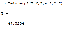
This problem can also be solved with MATLAB as it contains the predefined function interp2.
The MATLAB code is as shown below,
The output in the command window is,
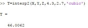
For more accuracy, the result can also be obtained from the bicubic interpolation as shown below,
Finally, the interpolation can also be implemented with the use of splines as shown below,
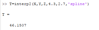
Hence, it can be concluded that the result is similar to that obtained from the calculation.
Want to see more full solutions like this?
Chapter 20 Solutions
Numerical Methods for Engineers


- At the start of a trip, the odometer on a car read 21,395. At the end of the trip, 13.5 hours later, the odometer read 22,125, Assume the scale on the odometer is in miles. What is the average speed the car traveled during this trip?arrow_forwardUse the table of values you made in part 4 of the example to find the limiting value of the average rate of change in velocity.arrow_forwardA piece shown by the shaded portion is to be cut from a square plate 128 millimeters on a side. a. Compute the area of the piece to be cut. Round the answer to the nearest square millimeter. b. After cutting the piece, determine the percentage of the plate that will be wasted.arrow_forward
- The average daily attendance for horror movies over the summers during the years 2007 to 2009 is documented in the table below. If the auditorium has an area of 2,025 ft^2, which of the following statements best describes the percent increase each year in terms of people per square foot of the auditorium? Year Number of Tickets Sold 2007 558 2008 623 2009 699 The movie theatre auditorium was more crowded in 2008 than in 2009. The largest annual percent increase in density occurred from 2008 to 2009. The smallest annual percent increase in density occurred from 2007 to 2008. The largest annual percent increase in density occurred from 2007 to 2008.arrow_forwardConsider the data sets below, determine if it is reasonable to assume that y is proportionalto x. If it is, approximate the constant of proportionality. If it is not, describe why thisassumption is not reasonable.arrow_forwardFind the measures of dispersion and interpret the resultsarrow_forward
 Mathematics For Machine TechnologyAdvanced MathISBN:9781337798310Author:Peterson, John.Publisher:Cengage Learning,
 Holt Mcdougal Larson Pre-algebra: Student Edition...AlgebraISBN:9780547587776Author:HOLT MCDOUGALPublisher:HOLT MCDOUGAL
 Functions and Change: A Modeling Approach to Coll...AlgebraISBN:9781337111348Author:Bruce Crauder, Benny Evans, Alan NoellPublisher:Cengage Learning
 Algebra & Trigonometry with Analytic GeometryAlgebraISBN:9781133382119Author:SwokowskiPublisher:Cengage
 Algebra: Structure And Method, Book 1AlgebraISBN:9780395977224Author:Richard G. Brown, Mary P. Dolciani, Robert H. Sorgenfrey, William L. ColePublisher:McDougal Littell