
ELEMENTARY STATISTICS(LL)(FD)
3rd Edition
ISBN: 9781260707458
Author: Navidi
Publisher: MCGRAW-HILL CUSTOM PUBLISHING
expand_more
expand_more
format_list_bulleted
Concept explainers
Videos
Textbook Question
Chapter 2.4, Problem 13E
College degrees: Both of the following time-series plots present the percentage of U.S. adults who have earned college degrees during the years 2007—20 15.
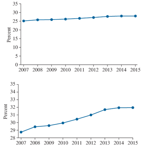
Which of the following statements is true and why?
- The percentage of U.S. adults with college degrees increased slightly between 2007 and 2015.
- The percentage of U.S. adults with college degrees increased considerably between 2007 and 2015.
Expert Solution & Answer
Want to see the full answer?
Check out a sample textbook solution
Students have asked these similar questions
B4. A company has collected and smoothened its historical yearly sales data of a product from
2015 up to 2021. The following table shows the sales and moving average figures.
Sales
Three-year moving
avcrage
Year
Five-ycar moving
avcrage
(S thousands)
2015
2016
326.0
324.0
E
367.4
2017
344.0
2018
383.0
371.0
2019
B.
389.0
2020
398.0
D
2021
428.0
Calculate the missing values of4, B, C, D. E and F(Correct to I decimal place).
B5. A lottery consists of 49 balls numbered 1 through 49 and 6 of them are drawn at random.
(a) You can pick 6 different numbers for a betting ticket. How many selections are possible?
(b) If prizes will be paid to those picking 4 to 6 drawn numbers, how many winning selections
are possible?
ర
Please solve all the questions below
Table #2.3.7 contains the value of the house and the amount of rental income in a year that the house brings in ("Capital and rental," 2013). Create a scatter plot and state if there is a relationship between the value of the house and the annual rental income.
Table #2.3.7: Data of House Value versus Rental
Value
Rental
Value
Rental
Value
Rental
Value
Rental
81000
6656
77000
4576
75000
7280
67500
6864
95000
7904
94000
8736
90000
6240
85000
7072
121000
12064
115000
7904
110000
7072
104000
7904
135000
8320
130000
9776
126000
6240
125000
7904
145000
8320
140000
9568
140000
9152
135000
7488
165000
13312
165000
8528
155000
7488
148000
8320
178000
11856
174000
10400
170000
9568
170000
12688
200000
12272
200000
10608
194000
11232
190000
8320
214000
8528
208000
10400
200000
10400
200000
8320
240000
10192…
Chapter 2 Solutions
ELEMENTARY STATISTICS(LL)(FD)
Ch. 2.1 - In Exercises 5-8, fill in each blank with the...Ch. 2.1 - In Exercises 5-8, fill in each blank with the...Ch. 2.1 - In Exercises 5-8, fill in each blank with the...Ch. 2.1 - In Exercises 5-8, fill in each blank with the...Ch. 2.1 - In Exercises 9—12, determine whether the...Ch. 2.1 - In Exercises 9—12, determine whether the...Ch. 2.1 - In Exercises 9—12, determine whether the...Ch. 2.1 - In Exercises 9—12, determine whether the...Ch. 2.1 - The following bar graph presents the average...Ch. 2.1 - The most common blood typing system divides human...
Ch. 2.1 - Following is a pie chart that presents the...Ch. 2.1 - Government spending: The following pie chart...Ch. 2.1 - U.S. population: The following side-by-side bar...Ch. 2.1 - Super Bowl: The following side-by-side bar graph...Ch. 2.1 - Smartphone sales: The following frequency...Ch. 2.1 - Popular video games: The following frequency...Ch. 2.1 - More smartphones: Using the data in Exercise 19:...Ch. 2.1 - More video games: Using the data in Exercise 20:...Ch. 2.1 - Hospital admissions: The following frequency...Ch. 2.1 - World population: Following are the populations of...Ch. 2.1 - Ages of video garners: The Nielsen Company...Ch. 2.1 - How secure is your job? In a survey, employed...Ch. 2.1 - Back up your data: In a survey commissioned by the...Ch. 2.1 - Education levels: The following frequency...Ch. 2.1 - Twitter followers: The following frequency...Ch. 2.1 - Music sales: The following frequency distribution...Ch. 2.1 - Keeping up with the Kardashians: The following...Ch. 2.1 - Bought a new car lately? The following table...Ch. 2.1 - Bought a new- truck lately? The following table...Ch. 2.1 - Happy Halloween: The following table presents...Ch. 2.1 - Native languages: The following frequency...Ch. 2.1 - Proportion of females: Following are the...Ch. 2.2 - Prob. 5ECh. 2.2 - In Exercises 5—8, fill in each blank with the...Ch. 2.2 - In Exercises 5—8, fill in each blank with the...Ch. 2.2 - In Exercises 5—8, fill in each blank with the...Ch. 2.2 - In Exercises 9—12, determine whether the...Ch. 2.2 - In Exercises 9—12, determine whether the...Ch. 2.2 - In Exercises 9—12, determine whether the...Ch. 2.2 - In Exercises 9—12, determine whether the...Ch. 2.2 - In Exercises 13—16, classify the histogram as...Ch. 2.2 - In Exercises 13—16, classify the histogram as...Ch. 2.2 - In Exercises 13—16, classify the histogram as...Ch. 2.2 - In Exercises 13—16, classify the histogram as...Ch. 2.2 - In Exercises 17 and 18, classify the histogram as...Ch. 2.2 - In Exercises 17 and 18, classify the histogram as...Ch. 2.2 - Student heights: The following frequency histogram...Ch. 2.2 - Trained rats: Forty rats were trained to run a...Ch. 2.2 - Cholesterol: The following histogram shows the...Ch. 2.2 - Blood pressure: The following histogram shows the...Ch. 2.2 - Olympic athletes: The following frequency...Ch. 2.2 - Hows the weather? The following relative frequency...Ch. 2.2 - Skewed which way? For which of the following data...Ch. 2.2 - Skewed which way? For which of the following data...Ch. 2.2 - Batting average: The following frequency...Ch. 2.2 - Batting average: The following frequency...Ch. 2.2 - Time spent playing video games: A sample of 200...Ch. 2.2 - Murder, she wrote: The following frequency...Ch. 2.2 - BMW prices: The following table presents the...Ch. 2.2 - Geysers: The geyser Old Faithful in Yellowstone...Ch. 2.2 - Hail to the chief: There have been 58 presidential...Ch. 2.2 - Internet radio: The following table presents the...Ch. 2.2 - Brothers and sisters: Thirty students in a...Ch. 2.2 - Cough, cough: The following table presents the...Ch. 2.2 - Prob. 37ECh. 2.2 - Prob. 38ECh. 2.2 - Prob. 39ECh. 2.2 - Prob. 40ECh. 2.2 - Frequency polygon: Using the data in Exercise 29:...Ch. 2.2 - Prob. 42ECh. 2.2 - Ogive: Using the data in Exercise 27: Compute the...Ch. 2.2 - Ogive: Using the data in Exercise 28: Compute the...Ch. 2.2 - Ogive: Using the data in Exercise 29: Compute the...Ch. 2.2 - Prob. 46ECh. 2.2 - Prob. 47ECh. 2.2 - Prob. 48ECh. 2.2 - Prob. 49ECh. 2.2 - Prob. 50ECh. 2.2 - Prob. 51ECh. 2.2 - Prob. 52ECh. 2.2 - Frequencies and relative frequencies: The...Ch. 2.3 - In Exercises 3—6, fill in each blank with the...Ch. 2.3 - In Exercises 3—6, fill in each blank with the...Ch. 2.3 - In Exercises 3—6, fill in each blank with the...Ch. 2.3 - In Exercises 3—6, fill in each blank with the...Ch. 2.3 - Prob. 7ECh. 2.3 - In Exercises 7—10, determine whether the...Ch. 2.3 - In Exercises 7—10, determine whether the...Ch. 2.3 - In Exercises 7—10, determine whether the...Ch. 2.3 - Construct a stem-and-leaf plot for the following...Ch. 2.3 - Construct a stem-and-leaf plot for the following...Ch. 2.3 - List the data in the following stem-and-leaf plot....Ch. 2.3 - List the data in the following stein-and-leaf...Ch. 2.3 - Construct a dotplot for the data in Exercise 11.Ch. 2.3 - Prob. 16ECh. 2.3 - BMW prices: The following table presents the...Ch. 2.3 - Hows the weather? The following table presents the...Ch. 2.3 - Air pollution: The following table presents...Ch. 2.3 - Technology salaries: The following table presents...Ch. 2.3 - Tennis and golf: Following are the ages of the...Ch. 2.3 - Pass the popcorn: Following are the running times...Ch. 2.3 - More weather: Construct a dotplot for the data in...Ch. 2.3 - Prob. 24ECh. 2.3 - Looking for a job: The following table presents...Ch. 2.3 - Prob. 26ECh. 2.3 - Military spending: The following table presents...Ch. 2.3 - Prob. 28ECh. 2.3 - Dining out: The following time-series plot...Ch. 2.3 - Prob. 30ECh. 2.3 - Prob. 31ECh. 2.3 - More gold: The following time series plot presents...Ch. 2.3 - Prob. 33ECh. 2.3 - Prob. 34ECh. 2.3 - Vote: The following time-series plot presents the...Ch. 2.3 - Arctic ice sheet: The following table presents the...Ch. 2.3 - Prob. 37ECh. 2.4 - In Exercises 3 and 4, fill in each blank with the...Ch. 2.4 - In Exercises 3 and 4, fill in each blank with the...Ch. 2.4 - CD sales decline: Sales of CDs have been declining...Ch. 2.4 - Music sales: The following time-series plot and...Ch. 2.4 - Stock market prices: The Dow Jones Industrial...Ch. 2.4 - Save your money: In 2007, U.S. residents saved...Ch. 2.4 - Ill take mine with mustard: The following bar...Ch. 2.4 - Stream or download? The following bar graph...Ch. 2.4 - Female senators: Of the 100 members of the United...Ch. 2.4 - Age at marriage: Data compiled by the U.S. Census...Ch. 2.4 - College degrees: Both of the following time-series...Ch. 2.4 - Food expenditures: Both of the following...Ch. 2.4 - Prob. 15ECh. 2 - Following is the list of letter grades for...Ch. 2 - Prob. 2CQCh. 2 - Construct a frequency bar graph for the data in...Ch. 2 - Prob. 4CQCh. 2 - Prob. 5CQCh. 2 - Prob. 6CQCh. 2 - Prob. 7CQCh. 2 - Prob. 8CQCh. 2 - Prob. 9CQCh. 2 - Prob. 10CQCh. 2 - Following are the prices (in dollars) for a sample...Ch. 2 - Prob. 12CQCh. 2 - Prob. 13CQCh. 2 - Prob. 14CQCh. 2 - Prob. 15CQCh. 2 - Trust your doctor: The General Social Survey...Ch. 2 - Internet browsers: The following relative...Ch. 2 - Prob. 3RECh. 2 - Prob. 4RECh. 2 - Prob. 5RECh. 2 - House freshmen: Newly elected members of the U.S....Ch. 2 - More freshmen: For the data in Exercise 6:...Ch. 2 - Royalty: Following are the ages at death for all...Ch. 2 - Prob. 9RECh. 2 - Prob. 10RECh. 2 - Prob. 11RECh. 2 - Prob. 12RECh. 2 - Prob. 13RECh. 2 - Prob. 14RECh. 2 - Prob. 15RECh. 2 - Explain why the frequency bar graph and the...Ch. 2 - Prob. 2WAICh. 2 - Prob. 3WAICh. 2 - Prob. 4WAICh. 2 - Prob. 5WAICh. 2 - In the chapter introduction, we presented gas...Ch. 2 - In the chapter introduction, we presented gas...Ch. 2 - In the chapter introduction, we presented gas...Ch. 2 - Prob. 4CSCh. 2 - In the chapter introduction, we presented gas...Ch. 2 - Prob. 6CSCh. 2 - In the chapter introduction, we presented gas...Ch. 2 - Prob. 8CSCh. 2 - In the chapter introduction, we presented gas...
Knowledge Booster


Learn more about
Need a deep-dive on the concept behind this application? Look no further. Learn more about this topic, statistics and related others by exploring similar questions and additional content below.Similar questions
- Table 6 shows the year and the number ofpeople unemployed in a particular city for several years. Determine whether the trend appears linear. If so, and assuming the trend continues, in what year will the number of unemployed reach 5 people?arrow_forwardDVD Player Sales The table shows the number of DVD players sold in a small electronics store in the years 2003-2013. Year DVD players sold 2003 495 2004 513 2005 410 2006 402 2007 520 2008 580 2009 631 2010 719 2011 624 2012 582 2013 635 aWhat was the average rate of change of sales between 2003 and 2013? bWhat was the average rate of change of sales between 2003 and 2004? cWhat was the average rate of change of sales between 2004 and 2005? dBetween which two successive years did DVD player sales increase most quickly? Decrease most quickly?arrow_forwardDVD Player sales The table shows the number of DVD play-ers sold in a small electronics store in the years 2003-2013. What was the average rate of change of sales between 2003 and 2013? Whatwas the average rate of change of sales between 2003 and 2004? What was the average rate of change of sales between 2004 and 2005? Between which two successive years did DVD player sales increase most quickly?arrow_forward
- Table 3 gives the annual sales (in millions of dollars) of a product from 1998 to 20006. What was the average rate of change of annual sales (a) between 2001 and 2002, and (b) between 2001 and 2004?arrow_forwardI'm running out of questions. Can I pay for 30 more extra?arrow_forwardB4. A company has collected and smoothened its historcal yearly sales data of a product from 2015 up to 2021. The following table shows the sales and moving average figures. Year Sales Three-year moving average Five-ycar moving average (S thousands) 2015 2016 326.0 324.0 E 367.4 2017 344.0 2018 383.0 371.0 E 2019 389.0 2020 398.0 D. 2021 428.0 Calculate the missing values of 4, B, C, D, E and F(Correct to I decimal place).arrow_forward
- The electric power consumed each month by a chemical plant is thought to be related to the average ambient temperature x1, the number of days in the month x2, the average product purity x3, and the tons of product produced x4. The past year's historical data are available and are presented in the following table. y 240 236 290 274 214 301 316 910 300 300 296 x1 25 31 45 60 00 65 99 72 14 X₂ 24 21 24 25 20 25 20 26 20 25 20 80 90 84 267 75 276 60 288 50 261 38 23 25 24 24 25 25 X3 91 90 88 00 87 91 94 2 87 DA 86 20 88 91 90 89 X₁ 100 95 110 88 94 99 97 96 110 105 100 98 Predict power consumption for a month in which x₁ =75°F, x₂ =24 days, x3 =90%, andx4 = 98 tons. Use 1 decimal place.arrow_forwardThe table below shows the number of state-registered automatic weapons and the murder rate for several Northwestern states. I 11.3 8.3 7.1 3.5 2.8 2.5 2.2 0.8 13.7 11.4 10.3 6.7 6.6 6 5.9 4.5 Y I = thousands of automatic weapons y = murders per 100,000 residents This data can be modeled by the equation = 0.89x + 3.88. Use this equation to answer the following. A) How many murders per 100,000 residents can be expected in a state with 5.7 thousand automatic weapons? Answer = Round to 3 decimal places. B) How many murders per 100,000 residents can be expected in a state with 3.3 thousand automatic weapons? Round to 3 decimal places. Answer = Question Help: Video Message instructor Submit Question Jump to Answerarrow_forwardIntergarated products Need to estimate its pc sales for the nextnext year. the most recent six years of revenue data for the companys line of xt personal computers and those of the industry, is found in the table below; Year XT PC Sales (000,000) All Industry PC Sales Revenue 1 2.4 4.6 2 5.9 8.6 3 15.5 10.7 4 27.8 14.8 5 35.9 18.5 6 38.1 19.4 a) Assuming that the sales data above are representative of sales expected next year , use time series regression analysis to forecast next years sales b) determine the correlation correlation for he ime forecast and interpret is meaning c) find the coefficient of determination for the time series forecast and intpret it s meaning d) perform a regression analysis between the annual sales revenues of XT Personal computers and all personal computers if the estimate of next years industry PC sales revenues is $21.9 billion? e) which independent variable should intergrated products coporation IPC choose for its forcasting of sales…arrow_forward
- An entrepreneur who owns and operates two businesses (A and B) would like to analyze their profitability. They would like your help in the analysis. They give you the annual net profit (in thousands of $) for each business from 2008-2020. Table 1: Annual Net Profits for Businesses A and B Business Year Profit Business Year Profit 2008 -50 2008 -10 2009 57 2009 30 2010 71 2010 27 2011 64 2011 22 2012 60 2012 21 2013 50 2013 20 A 2014 41 2014 24 2015 59 2015 24 2016 71 2016 32 2017 71 2017 36 2018 74 2018 37 019 81 20 40 2020 97 2020 49 a. Suppose you want to graph the distribution of profits. Explain why using only one stem- plot might not be optimal for the analysis. b. Describe the correct stemplot to use. Generate this stemplot. Explain your steps. What can you say about the distribution from this stemplot? c. When are stemplots useful? And why is that? d. Suppose that instead of having 26 observations you have 200 observations. What graph should you generate? e. What other type of…arrow_forwardThe median home value in South Dakota and Indiana (adjusted for inflation) are shown below: Year South Dakota 1950 32800 2000 79600 Indiana 37700 94300 If we assume that the house values are changing linearly, In which state have home values increased at a higher rate? Indiana If these trends were to continue, what would be the median home value in South Dakota in 2010? If we assume the linear trend existed before 1950 and continues after 2000, the two states' median house values will be (or were) equal in what year? (The answer might be absurd) The yeararrow_forwardThe table below shows the number of state-registered automatic weapons and the murder rate for several Northwestern states. x 11.5 8 6.6 3.5 2.9 2.3 2.7 0.4 y 13.6 10.5 9.7 6.8 6.2 5.7 6.5 4.2 * = thousands of automatic weapons y = murders per 100,000 residents This data can be modeled by the equation y = 0.84x + 3.9. Use this equation to answer the following; A) How many murders per 100,000 residents can be expected in a state with 5.6 thousand automatic weapons? Round to 3 decimal places. B) How many murders per 100,000 residents can be expected in a state with 9.8 thousand automatic weapons? Answer = Answer = Round to 3 decimal places.arrow_forward
arrow_back_ios
SEE MORE QUESTIONS
arrow_forward_ios
Recommended textbooks for you
 College AlgebraAlgebraISBN:9781305115545Author:James Stewart, Lothar Redlin, Saleem WatsonPublisher:Cengage Learning
 Algebra and Trigonometry (MindTap Course List)AlgebraISBN:9781305071742Author:James Stewart, Lothar Redlin, Saleem WatsonPublisher:Cengage Learning
 Glencoe Algebra 1, Student Edition, 9780079039897...AlgebraISBN:9780079039897Author:CarterPublisher:McGraw Hill
 Trigonometry (MindTap Course List)TrigonometryISBN:9781337278461Author:Ron LarsonPublisher:Cengage Learning
 Functions and Change: A Modeling Approach to Coll...AlgebraISBN:9781337111348Author:Bruce Crauder, Benny Evans, Alan NoellPublisher:Cengage Learning
College Algebra
Algebra
ISBN:9781305115545
Author:James Stewart, Lothar Redlin, Saleem Watson
Publisher:Cengage Learning
Algebra and Trigonometry (MindTap Course List)
Algebra
ISBN:9781305071742
Author:James Stewart, Lothar Redlin, Saleem Watson
Publisher:Cengage Learning
Glencoe Algebra 1, Student Edition, 9780079039897...
Algebra
ISBN:9780079039897
Author:Carter
Publisher:McGraw Hill
Trigonometry (MindTap Course List)
Trigonometry
ISBN:9781337278461
Author:Ron Larson
Publisher:Cengage Learning
Functions and Change: A Modeling Approach to Coll...
Algebra
ISBN:9781337111348
Author:Bruce Crauder, Benny Evans, Alan Noell
Publisher:Cengage Learning
The Shape of Data: Distributions: Crash Course Statistics #7; Author: CrashCourse;https://www.youtube.com/watch?v=bPFNxD3Yg6U;License: Standard YouTube License, CC-BY
Shape, Center, and Spread - Module 20.2 (Part 1); Author: Mrmathblog;https://www.youtube.com/watch?v=COaid7O_Gag;License: Standard YouTube License, CC-BY
Shape, Center and Spread; Author: Emily Murdock;https://www.youtube.com/watch?v=_YyW0DSCzpM;License: Standard Youtube License