Elementary Statistics ( 3rd International Edition ) Isbn:9781260092561
3rd Edition
ISBN: 9781259969454
Author: William Navidi Prof.; Barry Monk Professor
Publisher: McGraw-Hill Education
expand_more
expand_more
format_list_bulleted
Videos
Textbook Question
Chapter 2.4, Problem 14E
Food expenditures: Both of the following time-series plots present the percentage of income spent on food by U.S. residents for the years 1998 through 2014. (Source: U.S. Department of Agriculture)
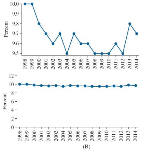
Which of the following statements is more accurate, and why?
(i) The percentage of income spent on food decreased considerably between 1998 and 2014.
(ii) The percentage of income spent on food decreased slightly between 1998 and 2014.
Expert Solution & Answer
Want to see the full answer?
Check out a sample textbook solution
Students have asked these similar questions
Movieflix, an online movie streaming service that offers a wide variety of award-winning TV shows, movies, animes, and documentaries, would like to determine the mathematical trend ofmemberships in order to project future needs.
MovieFlix - Advertising and Subscriptions
Year
Advertising Expenditure $ 000
Membership Subscriptions
2013
51
62
2014
58
68
2015
62
66
2016
65
66
2017
68
67
2018
76
72
2019
77
73
2020
78
72
2021
78
78
2022
84
73
2023
85
76
(i) Plot the scattergraph for the data.
Year Net Income Expenses 2013 $27,200 $19,800 2014. $23,700 $18,500 2015 $31,500 $23,900 2016 $33,600 $25,800 2017. $38,900 $29,200 2018 $41,400 $39,700 2019 $48,600 $37,300
a. What was Dana’s net income, in total for years 2013-19? b. In what year did Dana’s net income most exceed her expenses? c. Suggest a reasonable explanation for why Dana’s 2018 expenses were nearly as much as her income? (Use your business-minded logic, here. There are a number of possible explanations) d. What percent of Dana’s 2016 net income was needed for expenses? (to the nearest tenth of a %) e. What percent of her entire net income in these 7 years was Dana able to save? (nearest tenth of a %)
Question 5: A department store prints scratch-and-save discount coupons to distribute to its customers. The numbers for each present discount are shown in the table.
Present Discount
Number of Each type of discount Available
60%
50
50%
25000
30%
50000
10%
500,000
Determine the expected percent discount.
Chapter 2 Solutions
Elementary Statistics ( 3rd International Edition ) Isbn:9781260092561
Ch. 2.1 - In Exercises 5-8, fill in each blank with the...Ch. 2.1 - In Exercises 5-8, fill in each blank with the...Ch. 2.1 - In Exercises 5-8, fill in each blank with the...Ch. 2.1 - In Exercises 5-8, fill in each blank with the...Ch. 2.1 - In Exercises 9—12, determine whether the...Ch. 2.1 - In Exercises 9—12, determine whether the...Ch. 2.1 - In Exercises 9—12, determine whether the...Ch. 2.1 - In Exercises 9—12, determine whether the...Ch. 2.1 - The following bar graph presents the average...Ch. 2.1 - The most common blood typing system divides human...
Ch. 2.1 - Following is a pie chart that presents the...Ch. 2.1 - Government spending: The following pie chart...Ch. 2.1 - U.S. population: The following side-by-side bar...Ch. 2.1 - Super Bowl: The following side-by-side bar graph...Ch. 2.1 - Smartphone sales: The following frequency...Ch. 2.1 - Popular video games: The following frequency...Ch. 2.1 - More smartphones: Using the data in Exercise 19:...Ch. 2.1 - More video games: Using the data in Exercise 20:...Ch. 2.1 - Hospital admissions: The following frequency...Ch. 2.1 - World population: Following are the populations of...Ch. 2.1 - Ages of video garners: The Nielsen Company...Ch. 2.1 - How secure is your job? In a survey, employed...Ch. 2.1 - Back up your data: In a survey commissioned by the...Ch. 2.1 - Education levels: The following frequency...Ch. 2.1 - Twitter followers: The following frequency...Ch. 2.1 - Music sales: The following frequency distribution...Ch. 2.1 - Keeping up with the Kardashians: The following...Ch. 2.1 - Bought a new car lately? The following table...Ch. 2.1 - Bought a new- truck lately? The following table...Ch. 2.1 - Happy Halloween: The following table presents...Ch. 2.1 - Native languages: The following frequency...Ch. 2.1 - Proportion of females: Following are the...Ch. 2.2 - Prob. 5ECh. 2.2 - In Exercises 5—8, fill in each blank with the...Ch. 2.2 - In Exercises 5—8, fill in each blank with the...Ch. 2.2 - In Exercises 5—8, fill in each blank with the...Ch. 2.2 - In Exercises 9—12, determine whether the...Ch. 2.2 - In Exercises 9—12, determine whether the...Ch. 2.2 - In Exercises 9—12, determine whether the...Ch. 2.2 - In Exercises 9—12, determine whether the...Ch. 2.2 - In Exercises 13—16, classify the histogram as...Ch. 2.2 - In Exercises 13—16, classify the histogram as...Ch. 2.2 - In Exercises 13—16, classify the histogram as...Ch. 2.2 - In Exercises 13—16, classify the histogram as...Ch. 2.2 - In Exercises 17 and 18, classify the histogram as...Ch. 2.2 - In Exercises 17 and 18, classify the histogram as...Ch. 2.2 - Student heights: The following frequency histogram...Ch. 2.2 - Trained rats: Forty rats were trained to run a...Ch. 2.2 - Cholesterol: The following histogram shows the...Ch. 2.2 - Blood pressure: The following histogram shows the...Ch. 2.2 - Olympic athletes: The following frequency...Ch. 2.2 - Hows the weather? The following relative frequency...Ch. 2.2 - Skewed which way? For which of the following data...Ch. 2.2 - Skewed which way? For which of the following data...Ch. 2.2 - Batting average: The following frequency...Ch. 2.2 - Batting average: The following frequency...Ch. 2.2 - Time spent playing video games: A sample of 200...Ch. 2.2 - Murder, she wrote: The following frequency...Ch. 2.2 - BMW prices: The following table presents the...Ch. 2.2 - Geysers: The geyser Old Faithful in Yellowstone...Ch. 2.2 - Hail to the chief: There have been 58 presidential...Ch. 2.2 - Internet radio: The following table presents the...Ch. 2.2 - Brothers and sisters: Thirty students in a...Ch. 2.2 - Cough, cough: The following table presents the...Ch. 2.2 - Prob. 37ECh. 2.2 - Prob. 38ECh. 2.2 - Prob. 39ECh. 2.2 - Prob. 40ECh. 2.2 - Frequency polygon: Using the data in Exercise 29:...Ch. 2.2 - Prob. 42ECh. 2.2 - Ogive: Using the data in Exercise 27: Compute the...Ch. 2.2 - Ogive: Using the data in Exercise 28: Compute the...Ch. 2.2 - Ogive: Using the data in Exercise 29: Compute the...Ch. 2.2 - Prob. 46ECh. 2.2 - Prob. 47ECh. 2.2 - Prob. 48ECh. 2.2 - Prob. 49ECh. 2.2 - Prob. 50ECh. 2.2 - Prob. 51ECh. 2.2 - Prob. 52ECh. 2.2 - Frequencies and relative frequencies: The...Ch. 2.3 - In Exercises 3—6, fill in each blank with the...Ch. 2.3 - In Exercises 3—6, fill in each blank with the...Ch. 2.3 - In Exercises 3—6, fill in each blank with the...Ch. 2.3 - In Exercises 3—6, fill in each blank with the...Ch. 2.3 - Prob. 7ECh. 2.3 - In Exercises 7—10, determine whether the...Ch. 2.3 - In Exercises 7—10, determine whether the...Ch. 2.3 - In Exercises 7—10, determine whether the...Ch. 2.3 - Construct a stem-and-leaf plot for the following...Ch. 2.3 - Construct a stem-and-leaf plot for the following...Ch. 2.3 - List the data in the following stem-and-leaf plot....Ch. 2.3 - List the data in the following stein-and-leaf...Ch. 2.3 - Construct a dotplot for the data in Exercise 11.Ch. 2.3 - Prob. 16ECh. 2.3 - BMW prices: The following table presents the...Ch. 2.3 - Hows the weather? The following table presents the...Ch. 2.3 - Air pollution: The following table presents...Ch. 2.3 - Technology salaries: The following table presents...Ch. 2.3 - Tennis and golf: Following are the ages of the...Ch. 2.3 - Pass the popcorn: Following are the running times...Ch. 2.3 - More weather: Construct a dotplot for the data in...Ch. 2.3 - Prob. 24ECh. 2.3 - Looking for a job: The following table presents...Ch. 2.3 - Prob. 26ECh. 2.3 - Military spending: The following table presents...Ch. 2.3 - Prob. 28ECh. 2.3 - Dining out: The following time-series plot...Ch. 2.3 - Prob. 30ECh. 2.3 - Prob. 31ECh. 2.3 - More gold: The following time series plot presents...Ch. 2.3 - Prob. 33ECh. 2.3 - Prob. 34ECh. 2.3 - Vote: The following time-series plot presents the...Ch. 2.3 - Arctic ice sheet: The following table presents the...Ch. 2.3 - Prob. 37ECh. 2.4 - In Exercises 3 and 4, fill in each blank with the...Ch. 2.4 - In Exercises 3 and 4, fill in each blank with the...Ch. 2.4 - CD sales decline: Sales of CDs have been declining...Ch. 2.4 - Music sales: The following time-series plot and...Ch. 2.4 - Stock market prices: The Dow Jones Industrial...Ch. 2.4 - Save your money: In 2007, U.S. residents saved...Ch. 2.4 - Ill take mine with mustard: The following bar...Ch. 2.4 - Stream or download? The following bar graph...Ch. 2.4 - Female senators: Of the 100 members of the United...Ch. 2.4 - Age at marriage: Data compiled by the U.S. Census...Ch. 2.4 - College degrees: Both of the following time-series...Ch. 2.4 - Food expenditures: Both of the following...Ch. 2.4 - Prob. 15ECh. 2 - Following is the list of letter grades for...Ch. 2 - Prob. 2CQCh. 2 - Construct a frequency bar graph for the data in...Ch. 2 - Prob. 4CQCh. 2 - Prob. 5CQCh. 2 - Prob. 6CQCh. 2 - Prob. 7CQCh. 2 - Prob. 8CQCh. 2 - Prob. 9CQCh. 2 - Prob. 10CQCh. 2 - Following are the prices (in dollars) for a sample...Ch. 2 - Prob. 12CQCh. 2 - Prob. 13CQCh. 2 - Prob. 14CQCh. 2 - Prob. 15CQCh. 2 - Trust your doctor: The General Social Survey...Ch. 2 - Internet browsers: The following relative...Ch. 2 - Prob. 3RECh. 2 - Prob. 4RECh. 2 - Prob. 5RECh. 2 - House freshmen: Newly elected members of the U.S....Ch. 2 - More freshmen: For the data in Exercise 6:...Ch. 2 - Royalty: Following are the ages at death for all...Ch. 2 - Prob. 9RECh. 2 - Prob. 10RECh. 2 - Prob. 11RECh. 2 - Prob. 12RECh. 2 - Prob. 13RECh. 2 - Prob. 14RECh. 2 - Prob. 15RECh. 2 - Explain why the frequency bar graph and the...Ch. 2 - Prob. 2WAICh. 2 - Prob. 3WAICh. 2 - Prob. 4WAICh. 2 - Prob. 5WAICh. 2 - In the chapter introduction, we presented gas...Ch. 2 - In the chapter introduction, we presented gas...Ch. 2 - In the chapter introduction, we presented gas...Ch. 2 - Prob. 4CSCh. 2 - In the chapter introduction, we presented gas...Ch. 2 - Prob. 6CSCh. 2 - In the chapter introduction, we presented gas...Ch. 2 - Prob. 8CSCh. 2 - In the chapter introduction, we presented gas...
Knowledge Booster


Learn more about
Need a deep-dive on the concept behind this application? Look no further. Learn more about this topic, statistics and related others by exploring similar questions and additional content below.Similar questions
- The table below represents the monthly unemployment rates in the US from January of 2005 through May of 2016. Year Jan Feb Mar Apr May Jun Jul Aug Sep Oct Nov Dec 2005 5.3% 5.4% 5.2% 5.2% 5.1% 5.0% 5.0% 4.9% 5.0% 5.0% 5.0% 4.9% 2006 4.7% 4.8% 4.7% 4.7% 4.6% 4.6% 4.7% 4.7% 4.5% 4.4% 4.5% 4.4% 2007 4.6% 4.5% 4.4% 4.5% 4.4% 4.6% 4.7% 4.6% 4.7% 4.7% 4.7% 5.0% 2008 5.0% 4.9% 5.1% 5.0% 5.4% 5.6% 5.8% 6.1% 6.1% 6.5% 6.8% 7.3% 2009 7.8% 8.3% 8.7% 9.0% 9.4% 9.5% 9.5% 9.6% 9.8% 10.0% 9.9% 9.9% 2010 9.7% 9.8% 9.9% 9.9% 9.6% 9.4% 9.5% 9.5% 9.5% 9.5% 9.8% 9.4% 2011 9.1% 9.0% 9.0% 9.1% 9.0% 9.1% 9.0% 9.0% 9.0% 8.8% 8.6% 8.5% 2012 8.2% 8.3% 8.2% 8.2% 8.2% 8.2% 8.2% 8.1% 7.8% 7.8% 7.8% 7.9% 2013 7.9% 7.7% 7.5% 7.5% 7.5% 7.5% 7.3% 7.2%…arrow_forwardQuestion 3 The Bank of Canada is interested in studying the relationship between mortgage rates and median home prices. The data is provided below Year Interst rate Median home price 1988 10.30 183,800 1989 10.30 183,200 1990 10.10 174,900 1991 9.30 173,500 1992 8.40 172,900 1993 7.30 173,200 1994 8.40 173,200 1995 7.90 169,700 1996 7.60 174,500 1997 7.60 177,900 1998 6.90 188,100 1999 7.40 203,200 2000 8.10 230,200 2001 7.00 258,200 2002 6.50 309,800 2003 5.80 329,800 2004 5.80 431,000 2005 5.80 515,000 2006 6.40 537,000 2007 6.30 496,000 2008 6.00 352,000 2009 5.00 232,000 2010 4.70 291,700 2011 4.40 262,900 2012 3.60 299,200 2013 4.00 321,200 2014 4.10 373,500 2015 3.80 358,100 2016 3.60 382,500 2017 4.00 402,900 a) Estimate a…arrow_forwardYear Missouri Maine 1950 38800 29400 2000 89900 98700 If these trends were to continue, what would be the median home value in Missouri in 2010? c) If we assume the linear trend existed before 1950 and continues after 2000, the two states' median house values will be (or were) equal in what year?arrow_forward
- i. In the early 2000s interest rates were low so many homeowners refinanced their home mortgages. Linda is a mortgage officer at Maybank Savings and Loan. Below is the amount refinanced for twenty loans she processed last week. The data are reported in thousands of dollars and arranged from smallest to largest. 59.2 59.5 61.6 65.5 66.6 72.9 74.8 77.3 79.2 83.7 85.6 85.8 86.6 87.0 87.1 90.2 93.3 98.6 100.2 100.7 a. Find the mean, median, 1stquartile and 3rd quartile b. Draw a stem and leaf plot of the data using class width of 10 ii. The sales of Lexus automobiles in the Detroit area follow a Poisson distribution with a mean of 3 per day. a. What is the probability that no Lexus is sold on a particular day? b. What is the probability that for five consecutive days at least one Lexus is sold? please help me with this question. please do not reject itarrow_forwardAfter its move in 1990 to La Junta, Colorado, and its new initiatives, the DeBourgh Manufacturing Company began an upward climb of record sales. Suppose the figures shown here are the DeBourgh monthly sales figures from January 2001 through December 2009 (in $1,000s). a) Produce a time series plot. Are there any trends evident in the data? Does DeBourgh have a seasonal component to its sales? b) Deseasonalize the data using Multiplicative model with a 0.5 weighted moving average. Produce a time series plot of the deseasonalized data and add a trendline. c) Forecast the sales from January to December of the year 2010. d) Include a discussion of the general direction of sales and any seasonal tendencies that might be occurrinG Month 2001 2002 2003 2004 2005 2006 2007 2008 2009 January 139.7 165.1 177.8 228.6 266.7 431.8 381 431.8 495.3 February 114.3 177.8 203.2 254 317.5 457.2 406.4 444.5 533.4 March 101.6 177.8 228.6 266.7 368.3 457.2 431.8 495.3 635 April 152.4 203.2…arrow_forwardAn electronic appliance manufacturer wants to know if there is a relationship between percentage change in deposable personal income which is reported quarterly by the government, and the percentage change in appliances sold by the manufacturer following same years of quarterly data. Brenda Chee and Clarence Paulus lead an analyst team has obtained data for the past 10 quarters. (Hint: Provides your answers in two decimal points) Quarter Percent change in income Percent Change in appliance sold Quarter Percent change in income Percent change in appliance sold 1 -2.3 -2.5 6 -1.0 1.0 2 -1.5 -1.0 7 0.7 1.4 3 2.8 7.4 8 5.2 3.4 4 0.5 2.6 9 -2.5 -0.5 5 4.6 8.5 10 1.7 1.8 (a) What forecasting model should be used for this data. Why?(5(b) Develop the forecasting model that you have proposed in (a).(c) Compute the relationship for these data. In your opinion, is the relationship between independentvariable…arrow_forward
- Given information: Monthly Household Spending ($) Annual Household Income ($) HouseholdSize 4016 54000 3 3159 30000 2 5100 32000 4 4742 50000 5 1864 31000 2 4070 55000 2 2731 37000 1 3348 40000 2 4764 66000 4 4110 51000 3 4208 25000 3 4219 48000 4 2477 27000 1 2514 33000 2 4214 65000 3 4965 63000 4 4412 42000 6 2448 21000 2 2995 44000 1 4171 37000 5 5678 62000 6 3623 21000 3 5301 55000 7 3020 42000 2 4828 41000 7 5573 54000 6 2583 30000 1 3866 48000 2 3586 34000 5 5037 67000 4 3605 50000 2 5345 67000 5 5370 55000 6 3890 52000 2 4705 62000 3 4157 64000 2 3579 22000 3 3890 29000 4 2972 39000 2 3121 35000 1 4183 39000 4 3730 54000 3 4127 23000 6 2921 27000 2 4603 26000 7 4273 61000 2 3067 30000 2 3074 22000 4 4820 46000 5 5149 66000 4 EXCEL (Data Analysis) output: SUMMARY OUTPUT Regression Statistics Multiple R 0.908603921 R…arrow_forwardA manufacturer’s contribution margin income statement for the year follows. Prepare contribution margin income statements for each of the two separate cases below. Unit selling price decreases by 5% and units sold and produced increase by 8%. Hint: A unit increase has both a sales and costs impact. Fixed costs increase by $20,000, variable costs per unit decrease by $2, and units sold and produced increase by 500 Use the table below to figure out the Sales, Variable Cost, Contribution Margin, Fixed Cost, and Income (loss) of each question.arrow_forwardQuestion 3 The Bank of Canada is interested in studying the relationship between mortgage rates and median home prices. The data is provided below Year interest rate (%) 1988 10.30 1989 10.30 1990 10.10 1991 9.30 1992 8.40 1993 7.30 1994 8.40 1995 7.90 1996 7.60 1997 7.60 1998 6.90 1999 7.40 2000 8.10 2001 7.00 2002 6.50 2003 5.80 2004 5.80 2005 5.80 2006 6.40 2007 6.30 2008 6.00 2009 5.00 2010 4.70 2011 4.40 2012 3.60 2013 4.00 2014 4.10 2015 3.80 2016 3.60 2017 4.00 Median home price $183,800 $183,200 $174,900 $173,500 $172,900 $173,200 $173,200 $169,700 $174,500 $177,900 $188,100 $203,200 $230,200 $258,200 $309,800 $329,800 $431,000 $515,000 $537,000 $496,000 $352,000 $232,000 $291,700 $262,900 $299,200 $321,200 $373,500 $358,100 $382,500 $402,900 a) Estimate a simple linear regression model and find the value of the parameters for the estimation of mortgage rates and the median home price b) Interpret the intercept and the slope coefficients…arrow_forward
- The Badrutt’s Palace Hotel St. Moritz which is one of the best Alpine hotels in Switzerland has provided you with their quarterly bookings data over the last 6 years as follows: Year Quarter-1 (Demand in units) Quarter-2 (Demand in units) Quarter-3 (Demand in units) Quarter-4 (Demand in units) 2018 45,000 22,000 64,000 33,000 2019 48,000 27,000 74,000 41,000 2020 52,000 32,000 83,000 46,000 2021 57,000 35,000 94,000 52,000 2022 61,000 42,000 104,000 56,000 2023 67,000 49,000 120,000 61,000 Required: i) Calculate the seasonal indices for each season using multiplicative index ii) Forecast the demand for each season of the year 2024 given that the annual demand forecast is 324,000 units. iii) Deseasonalize the actual demand data (2018-2023) above using the seasonal indices obtained in (a) above. iv) Generate OLS equation using the Deseasonalized data in (iii) above (in thousand units)arrow_forwardThe following information on maintenance and repair costs and revenues for the last two years is available from the accounting records at Arnie’s Arcade & Video Palace. Arnie has asked you to help him understand the relation between business volume and maintenance and repair cost. Month Maintenance and Repair Cost ($000) Revenues ($000) July $2.31 $59.00 August 3.28 53.00 September 2.80 49.00 October 2.21 65.00 November 2.30 77.00 December 1.14 105.00 January 3.12 45.00 February 3.16 51.00 March 3.02 61.00 April 2.98 63.00 May 2.04 67.00 June 1.78 79.00 July 2.60 73.00 August 2.02 67.00 September 2.57 75.00 October 2.38 77.00 November 1.43 87.00 December 0.76 117.00 January 2.58 61.00 February 2.28 63.00 March 1.69 83.00 April 1.95 87.00 May 1.95 73.00 June 1.33 69.00 Required: Using Excel, estimate a linear regression with maintenance and repair cost as the dependent variable and revenue as the independent variable.…arrow_forwardCompanies are devoting time and energy to promote recycling. A major recycling company found some old documents that present the recorded amount of cell phone collected over a span of eight years. Year Cellular Telephones Collected (in millions) 2009 2.2 2010 2.6 2011 2.9 2012 3.4 2013 3.1 2014 4.2 2015 4.9 2016 5.3 Part a) Develop a time series plot with Year on the X axis and Cellular Telephones Collected on the Y axis. Part b) Does there appear to be a relationship between time and cellular telephones collected?arrow_forward
arrow_back_ios
arrow_forward_ios
Recommended textbooks for you
 MATLAB: An Introduction with ApplicationsStatisticsISBN:9781119256830Author:Amos GilatPublisher:John Wiley & Sons Inc
 Probability and Statistics for Engineering and th...StatisticsISBN:9781305251809Author:Jay L. DevorePublisher:Cengage Learning
 Statistics for The Behavioral Sciences (MindTap C...StatisticsISBN:9781305504912Author:Frederick J Gravetter, Larry B. WallnauPublisher:Cengage Learning
 Elementary Statistics: Picturing the World (7th E...StatisticsISBN:9780134683416Author:Ron Larson, Betsy FarberPublisher:PEARSON
 The Basic Practice of StatisticsStatisticsISBN:9781319042578Author:David S. Moore, William I. Notz, Michael A. FlignerPublisher:W. H. Freeman
 Introduction to the Practice of StatisticsStatisticsISBN:9781319013387Author:David S. Moore, George P. McCabe, Bruce A. CraigPublisher:W. H. Freeman
MATLAB: An Introduction with Applications
Statistics
ISBN:9781119256830
Author:Amos Gilat
Publisher:John Wiley & Sons Inc
Probability and Statistics for Engineering and th...
Statistics
ISBN:9781305251809
Author:Jay L. Devore
Publisher:Cengage Learning
Statistics for The Behavioral Sciences (MindTap C...
Statistics
ISBN:9781305504912
Author:Frederick J Gravetter, Larry B. Wallnau
Publisher:Cengage Learning
Elementary Statistics: Picturing the World (7th E...
Statistics
ISBN:9780134683416
Author:Ron Larson, Betsy Farber
Publisher:PEARSON
The Basic Practice of Statistics
Statistics
ISBN:9781319042578
Author:David S. Moore, William I. Notz, Michael A. Fligner
Publisher:W. H. Freeman
Introduction to the Practice of Statistics
Statistics
ISBN:9781319013387
Author:David S. Moore, George P. McCabe, Bruce A. Craig
Publisher:W. H. Freeman
What Are Research Ethics?; Author: HighSchoolScience101;https://www.youtube.com/watch?v=nX4c3V23DZI;License: Standard YouTube License, CC-BY
What is Ethics in Research - ethics in research (research ethics); Author: Chee-Onn Leong;https://www.youtube.com/watch?v=W8Vk0sXtMGU;License: Standard YouTube License, CC-BY