Concept explainers
(a)
The histogram frequency distribution, cumulative percentage distribution for each set of data and average speed.
Answer to Problem 10P
Explanation of Solution
Given:
Significance level of

Formula used:
Calculation:
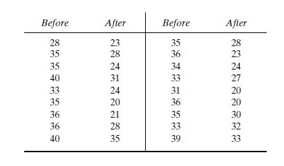
Before an increase in speed enforcement activities:
The speed ranges from 28 to 40 mi/h giving a speed range of 12. For five classes, the range per class is 2.4 mi/h. A frequency distribution table can then be prepared, as shown below in which the speed classes are listed in column 1 and the mid-values are in column 2. The number of observations for each class is listed in column 3 and the cumulative percentages of all observations are listed in column 6.
| 1 | 2 | 3 | 4 | 5 | 6 | 7 |
| Speed class (mi/h) | Class mid-value | Class frequency, | Percentage of class frequency | Cumulative percentage of class frequency | ||
| 28-30 | 29 | 4 | 116 | 13 | 13 | 139.24 |
| 31-33 | 32 | 5 | 160 | 17 | 30 | 42.05 |
| 34-36 | 35 | 12 | 420 | 40 | 70 | 0.12 |
| 37-39 | 38 | 6 | 228 | 20 | 90 | 57.66 |
| 40-42 | 41 | 3 | 123 | 10 | 100 | 111.63 |
| Total | 30 | 1047 | 350.7 |
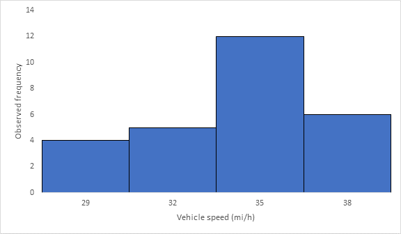
Below Figure shows the frequency histogram for the data shown in above Table. The values in columns 2 and 3 of Table are used to draw the frequency histogram, where the abscissa represents the speeds and the ordinate the observed frequency in each class.

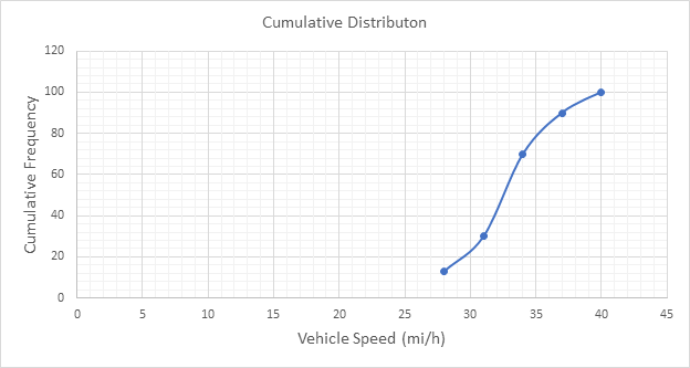
Below Figure shows the cumulative frequency distribution curve for the data given. In this case, the cumulative percentages in column 6 of above Table are plotted against the upper limit of each corresponding speed class. This curve gives the percentage of vehicles that are traveling at or below a given speed.

Determine the arithmetic mean speed:
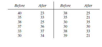
After an increase in speed enforcement activities:
The speed ranges from 20 to 37 mi/h giving a speed range of 17. For six classes, the range per class is 2.83 mi/h. A frequency distribution table can then be prepared, as shown below in which the speed classes are listed in column 1 and the mid-values are in column 2. The number of observations for each class is listed in column 3 and the cumulative percentages of all observations are listed in column 6.
| 1 | 2 | 3 | 4 | 5 | 6 | 7 |
| Speed class (mi/h) | Class mid-value | Class frequency, | Percentage of class frequency | Cumulative percentage of class frequency | ||
| 20-22 | 21 | 6 | 126 | 20 | 20 | 253.5 |
| 23-25 | 24 | 8 | 192 | 27 | 47 | 98 |
| 26-28 | 27 | 4 | 108 | 13 | 60 | 1 |
| 29-31 | 30 | 3 | 90 | 10 | 70 | 18.75 |
| 32-34 | 33 | 5 | 165 | 17 | 87 | 151.25 |
| 35-37 | 36 | 4 | 144 | 13 | 100 | 289 |
| Total | 30 | 825 | 811.5 |
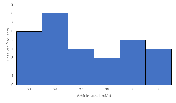
Below Figure shows the frequency histogram for the data shown in above Table. The values in columns 2 and 3 of Table are used to draw the frequency histogram, where the abscissa represents the speeds and the ordinate the observed frequency in each class.

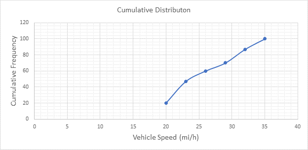
Below Figure shows the cumulative frequency distribution curve for the data given. In this case, the cumulative percentages in column 6 of above Table are plotted against the upper limit of each corresponding speed class. This curve gives the percentage of vehicles that are traveling at or below a given speed.

Determine the arithmetic mean speed:
Conclusion:
The average speeds of each set of data are 34.9 and 27.5 mi/h respectively.
(b)
The histogram frequency distribution, cumulative percentage distribution for each set of data and 85th percentile speed.
Answer to Problem 10P
Explanation of Solution
Given:
Significance level of

Calculation:
Before an increase in speed enforcement activities:
The speed ranges from 28 to 40 mi/h giving a speed range of 12. For five classes, the range per class is 2.4 mi/h. A frequency distribution table can then be prepared, as shown below in which the speed classes are listed in column 1 and the mid-values are in column 2. The number of observations for each class is listed in column 3 and the cumulative percentages of all observations are listed in column 6.
| 1 | 2 | 3 | 4 | 5 | 6 | 7 |
| Speed class (mi/h) | Class mid-value | Class frequency, | Percentage of class frequency | Cumulative percentage of class frequency | ||
| 28-30 | 29 | 4 | 116 | 13 | 13 | 139.24 |
| 31-33 | 32 | 5 | 160 | 17 | 30 | 42.05 |
| 34-36 | 35 | 12 | 420 | 40 | 70 | 0.12 |
| 37-39 | 38 | 6 | 228 | 20 | 90 | 57.66 |
| 40-42 | 41 | 3 | 123 | 10 | 100 | 111.63 |
| Total | 30 | 1047 | 350.7 |
Below Figure shows the frequency histogram for the data shown in above Table. The values in columns 2 and 3 of Table are used to draw the frequency histogram, where the abscissa represents the speeds and the ordinate the observed frequency in each class.

Below Figure shows the cumulative frequency distribution curve for the data given. In this case, the cumulative percentages in column 6 of above Table are plotted against the upper limit of each corresponding speed class. This curve gives the percentage of vehicles that are traveling at or below a given speed.

The 85th-percentile speed is obtained from the cumulative frequency distribution curve as 36 mi/h.
After an increase in speed enforcement activities:
The speed ranges from 20 to 37 mi/h giving a speed range of 17. For six classes, the range per class is 2.83 mi/h. A frequency distribution table can then be prepared, as shown below in which the speed classes are listed in column 1 and the mid-values are in column 2. The number of observations for each class is listed in column 3 and the cumulative percentages of all observations are listed in column 6.
| 1 | 2 | 3 | 4 | 5 | 6 | 7 |
| Speed class (mi/h) | Class mid-value | Class frequency, | Percentage of class frequency | Cumulative percentage of class frequency | ||
| 20-22 | 21 | 6 | 126 | 20 | 20 | 253.5 |
| 23-25 | 24 | 8 | 192 | 27 | 47 | 98 |
| 26-28 | 27 | 4 | 108 | 13 | 60 | 1 |
| 29-31 | 30 | 3 | 90 | 10 | 70 | 18.75 |
| 32-34 | 33 | 5 | 165 | 17 | 87 | 151.25 |
| 35-37 | 36 | 4 | 144 | 13 | 100 | 289 |
| Total | 30 | 825 | 811.5 |
Below Figure shows the frequency histogram for the data shown in above Table. The values in columns 2 and 3 of Table are used to draw the frequency histogram, where the abscissa represents the speeds and the ordinate the observed frequency in each class.

Below Figure shows the cumulative frequency distribution curve for the data given. In this case, the cumulative percentages in column 6 of above Table are plotted against the upper limit of each corresponding speed class. This curve gives the percentage of vehicles that are traveling at or below a given speed.

The 85th-percentile speed is obtained from the cumulative frequency distribution curve as 31.5 mi/h.
Conclusion:
The 85th-percentile speed for each set of data are 36 and 31.5 mi/h respectively.
(c)
The histogram frequency distribution, cumulative percentage distribution for each set of data and 15th percentile speed.
Answer to Problem 10P
Explanation of Solution
Given:
Significance level of


Calculation:
Before an increase in speed enforcement activities:
The speed ranges from 28 to 40 mi/h giving a speed range of 12. For five classes, the range per class is 2.4 mi/h. A frequency distribution table can then be prepared, as shown below in which the speed classes are listed in column 1 and the mid-values are in column 2. The number of observations for each class is listed in column 3 and the cumulative percentages of all observations are listed in column 6.
| 1 | 2 | 3 | 4 | 5 | 6 | 7 |
| Speed class (mi/h) | Class mid-value | Class frequency, | Percentage of class frequency | Cumulative percentage of class frequency | ||
| 28-30 | 29 | 4 | 116 | 13 | 13 | 139.24 |
| 31-33 | 32 | 5 | 160 | 17 | 30 | 42.05 |
| 34-36 | 35 | 12 | 420 | 40 | 70 | 0.12 |
| 37-39 | 38 | 6 | 228 | 20 | 90 | 57.66 |
| 40-42 | 41 | 3 | 123 | 10 | 100 | 111.63 |
| Total | 30 | 1047 | 350.7 |
Below Figure shows the frequency histogram for the data shown in above Table. The values in columns 2 and 3 of Table are used to draw the frequency histogram, where the abscissa represents the speeds and the ordinate the observed frequency in each class.
Below Figure shows the cumulative frequency distribution curve for the data given. In this case, the cumulative percentages in column 6 of above Table are plotted against the upper limit of each corresponding speed class. This curve gives the percentage of vehicles that are traveling at or below a given speed.

The 15th-percentile speed is obtained from the cumulative frequency distribution curve as 28.5 mi/h.
After an increase in speed enforcement activities:
The speed ranges from 20 to 37 mi/h giving a speed range of 17. For six classes, the range per class is 2.83 mi/h. A frequency distribution table can then be prepared, as shown below in which the speed classes are listed in column 1 and the mid-values are in column 2. The number of observations for each class is listed in column 3 and the cumulative percentages of all observations are listed in column 6.
| 1 | 2 | 3 | 4 | 5 | 6 | 7 |
| Speed class (mi/h) | Class mid-value | Class frequency, | Percentage of class frequency | Cumulative percentage of class frequency | ||
| 20-22 | 21 | 6 | 126 | 20 | 20 | 253.5 |
| 23-25 | 24 | 8 | 192 | 27 | 47 | 98 |
| 26-28 | 27 | 4 | 108 | 13 | 60 | 1 |
| 29-31 | 30 | 3 | 90 | 10 | 70 | 18.75 |
| 32-34 | 33 | 5 | 165 | 17 | 87 | 151.25 |
| 35-37 | 36 | 4 | 144 | 13 | 100 | 289 |
| Total | 30 | 825 | 811.5 |
Below Figure shows the frequency histogram for the data shown in above Table. The values in columns 2 and 3 of Table are used to draw the frequency histogram, where the abscissa represents the speeds and the ordinate the observed frequency in each class.
Below Figure shows the cumulative frequency distribution curve for the data given. In this case, the cumulative percentages in column 6 of above Table are plotted against the upper limit of each corresponding speed class. This curve gives the percentage of vehicles that are traveling at or below a given speed.
The 15th-percentile speed is obtained from the cumulative frequency distribution curve as 0 mi/h.
Conclusion:
The 15th-percentile speed for each set of data are 28.5 and 0 mi/h respectively.
(d)
The histogram frequency distribution, cumulative percentage distribution for each set of data and mode.
Answer to Problem 10P
35 mi/h and 24 mi/h
Explanation of Solution
Given:
Significance level of


Calculation:
Before an increase in speed enforcement activities:
The speed ranges from 28 to 40 mi/h giving a speed range of 12. For five classes, the range per class is 2.4 mi/h. A frequency distribution table can then be prepared, as shown below in which the speed classes are listed in column 1 and the mid-values are in column 2. The number of observations for each class is listed in column 3 and the cumulative percentages of all observations are listed in column 6.
| 1 | 2 | 3 | 4 | 5 | 6 | 7 |
| Speed class (mi/h) | Class mid-value | Class frequency, | Percentage of class frequency | Cumulative percentage of class frequency | ||
| 28-30 | 29 | 4 | 116 | 13 | 13 | 139.24 |
| 31-33 | 32 | 5 | 160 | 17 | 30 | 42.05 |
| 34-36 | 35 | 12 | 420 | 40 | 70 | 0.12 |
| 37-39 | 38 | 6 | 228 | 20 | 90 | 57.66 |
| 40-42 | 41 | 3 | 123 | 10 | 100 | 111.63 |
| Total | 30 | 1047 | 350.7 |
Below Figure shows the frequency histogram for the data shown in above Table. The values in columns 2 and 3 of Table are used to draw the frequency histogram, where the abscissa represents the speeds and the ordinate the observed frequency in each class.

Below Figure shows the cumulative frequency distribution curve for the data given. In this case, the cumulative percentages in column 6 of above Table are plotted against the upper limit of each corresponding speed class. This curve gives the percentage of vehicles that are traveling at or below a given speed.

The mode or modal speed is obtained from the frequency histogram as 35 mi/h
After an increase in speed enforcement activities:
The speed ranges from 20 to 37 mi/h giving a speed range of 17. For six classes, the range per class is 2.83 mi/h. A frequency distribution table can then be prepared, as shown below in which the speed classes are listed in column 1 and the mid-values are in column 2. The number of observations for each class is listed in column 3 and the cumulative percentages of all observations are listed in column 6.
| 1 | 2 | 3 | 4 | 5 | 6 | 7 |
| Speed class (mi/h) | Class mid-value | Class frequency, | Percentage of class frequency | Cumulative percentage of class frequency | ||
| 20-22 | 21 | 6 | 126 | 20 | 20 | 253.5 |
| 23-25 | 24 | 8 | 192 | 27 | 47 | 98 |
| 26-28 | 27 | 4 | 108 | 13 | 60 | 1 |
| 29-31 | 30 | 3 | 90 | 10 | 70 | 18.75 |
| 32-34 | 33 | 5 | 165 | 17 | 87 | 151.25 |
| 35-37 | 36 | 4 | 144 | 13 | 100 | 289 |
| Total | 30 | 825 | 811.5 |
Below Figure shows the frequency histogram for the data shown in above Table. The values in columns 2 and 3 of Table are used to draw the frequency histogram, where the abscissa represents the speeds and the ordinate the observed frequency in each class.

Below Figure shows the cumulative frequency distribution curve for the data given. In this case, the cumulative percentages in column 6 of above Table are plotted against the upper limit of each corresponding speed class. This curve gives the percentage of vehicles that are traveling at or below a given speed.

The mode or modal speed is obtained from the frequency histogram as 24 mi/h.
Conclusion:
The mode for each set of data are 35 and 24 mi/h respectively.
(e)
The histogram frequency distribution, cumulative percentage distribution for each set of data and median.
Answer to Problem 10P
32.5 and 23.5 mi/h
Explanation of Solution
Given:
Significance level of


Calculation:
Before an increase in speed enforcement activities:
The speed ranges from 28 to 40 mi/h giving a speed range of 12. For five classes, the range per class is 2.4 mi/h. A frequency distribution table can then be prepared, as shown below in which the speed classes are listed in column 1 and the mid-values are in column 2. The number of observations for each class is listed in column 3 and the cumulative percentages of all observations are listed in column 6.
| 1 | 2 | 3 | 4 | 5 | 6 | 7 |
| Speed class (mi/h) | Class mid-value | Class frequency, | Percentage of class frequency | Cumulative percentage of class frequency | ||
| 28-30 | 29 | 4 | 116 | 13 | 13 | 139.24 |
| 31-33 | 32 | 5 | 160 | 17 | 30 | 42.05 |
| 34-36 | 35 | 12 | 420 | 40 | 70 | 0.12 |
| 37-39 | 38 | 6 | 228 | 20 | 90 | 57.66 |
| 40-42 | 41 | 3 | 123 | 10 | 100 | 111.63 |
| Total | 30 | 1047 | 350.7 |
Below Figure shows the frequency histogram for the data shown in above Table. The values in columns 2 and 3 of Table are used to draw the frequency histogram, where the abscissa represents the speeds and the ordinate the observed frequency in each class.

Below Figure shows the cumulative frequency distribution curve for the data given. In this case, the cumulative percentages in column 6 of above Table are plotted against the upper limit of each corresponding speed class. This curve gives the percentage of vehicles that are traveling at or below a given speed.

The median speed is obtained from the cumulative frequency distribution curve as 32.5 mi/h which is the 50th percentile speed.
After an increase in speed enforcement activities:
The speed ranges from 20 to 37 mi/h giving a speed range of 17. For six classes, the range per class is 2.83 mi/h. A frequency distribution table can then be prepared, as shown below in which the speed classes are listed in column 1 and the mid-values are in column 2. The number of observations for each class is listed in column 3 and the cumulative percentages of all observations are listed in column 6.
| 1 | 2 | 3 | 4 | 5 | 6 | 7 |
| Speed class (mi/h) | Class mid-value | Class frequency, | Percentage of class frequency | Cumulative percentage of class frequency | ||
| 20-22 | 21 | 6 | 126 | 20 | 20 | 253.5 |
| 23-25 | 24 | 8 | 192 | 27 | 47 | 98 |
| 26-28 | 27 | 4 | 108 | 13 | 60 | 1 |
| 29-31 | 30 | 3 | 90 | 10 | 70 | 18.75 |
| 32-34 | 33 | 5 | 165 | 17 | 87 | 151.25 |
| 35-37 | 36 | 4 | 144 | 13 | 100 | 289 |
| Total | 30 | 825 | 811.5 |
Below Figure shows the frequency histogram for the data shown in above Table. The values in columns 2 and 3 of Table are used to draw the frequency histogram, where the abscissa represents the speeds and the ordinate the observed frequency in each class.

Below Figure shows the cumulative frequency distribution curve for the data given. In this case, the cumulative percentages in column 6 of above Table are plotted against the upper limit of each corresponding speed class. This curve gives the percentage of vehicles that are traveling at or below a given speed.

The median speed is obtained from the cumulative frequency distribution curve as 23.5 mi/h which is the 50th percentile speed.
Conclusion:
The median speed for each set of data are 32.5 and 23.5 mi/h respectively.
(f)
The histogram frequency distribution, cumulative percentage distribution for each set of data and pace.
Answer to Problem 10P
32 to 39 mi/h and 27 to 36 mi/h
Explanation of Solution
Given:
Significance level of


Calculation:
Before an increase in speed enforcement activities:
The speed ranges from 28 to 40 mi/h giving a speed range of 12. For five classes, the range per class is 2.4 mi/h. A frequency distribution table can then be prepared, as shown below in which the speed classes are listed in column 1 and the mid-values are in column 2. The number of observations for each class is listed in column 3 and the cumulative percentages of all observations are listed in column 6.
| 1 | 2 | 3 | 4 | 5 | 6 | 7 |
| Speed class (mi/h) | Class mid-value | Class frequency, | Percentage of class frequency | Cumulative percentage of class frequency | ||
| 28-30 | 29 | 4 | 116 | 13 | 13 | 139.24 |
| 31-33 | 32 | 5 | 160 | 17 | 30 | 42.05 |
| 34-36 | 35 | 12 | 420 | 40 | 70 | 0.12 |
| 37-39 | 38 | 6 | 228 | 20 | 90 | 57.66 |
| 40-42 | 41 | 3 | 123 | 10 | 100 | 111.63 |
| Total | 30 | 1047 | 350.7 |
Below Figure shows the frequency histogram for the data shown in above Table. The values in columns 2 and 3 of Table are used to draw the frequency histogram, where the abscissa represents the speeds and the ordinate the observed frequency in each class.

Below Figure shows the cumulative frequency distribution curve for the data given. In this case, the cumulative percentages in column 6 of above Table are plotted against the upper limit of each corresponding speed class. This curve gives the percentage of vehicles that are traveling at or below a given speed.
Below figure shows the frequency distribution curve for the data given. In this case, a curve showing percentage of observations against speed is drawn by plotting values from column 5 of above Table against the corresponding values in column 2. The total area under this curve is one or 100 percent.
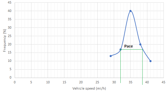
The pace is obtained from the frequency distribution curve above as 32 to 39 mi/h.
After an increase in speed enforcement activities:
The speed ranges from 20 to 37 mi/h giving a speed range of 17. For six classes, the range per class is 2.83 mi/h. A frequency distribution table can then be prepared, as shown below in which the speed classes are listed in column 1 and the mid-values are in column 2. The number of observations for each class is listed in column 3 and the cumulative percentages of all observations are listed in column 6.
| 1 | 2 | 3 | 4 | 5 | 6 | 7 |
| Speed class (mi/h) | Class mid-value | Class frequency, | Percentage of class frequency | Cumulative percentage of class frequency | ||
| 20-22 | 21 | 6 | 126 | 20 | 20 | 253.5 |
| 23-25 | 24 | 8 | 192 | 27 | 47 | 98 |
| 26-28 | 27 | 4 | 108 | 13 | 60 | 1 |
| 29-31 | 30 | 3 | 90 | 10 | 70 | 18.75 |
| 32-34 | 33 | 5 | 165 | 17 | 87 | 151.25 |
| 35-37 | 36 | 4 | 144 | 13 | 100 | 289 |
| Total | 30 | 825 | 811.5 |
Below Figure shows the frequency histogram for the data shown in above Table. The values in columns 2 and 3 of Table are used to draw the frequency histogram, where the abscissa represents the speeds and the ordinate the observed frequency in each class.

Below Figure shows the cumulative frequency distribution curve for the data given. In this case, the cumulative percentages in column 6 of above Table are plotted against the upper limit of each corresponding speed class. This curve gives the percentage of vehicles that are traveling at or below a given speed.

Below figure shows the frequency distribution curve for the data given. In this case, a curve showing percentage of observations against speed is drawn by plotting values from column 5 of above Table against the corresponding values in column 2. The total area under this curve is one or 100 percent.
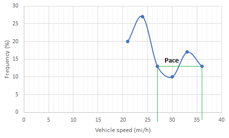
The pace is obtained from the frequency distribution curve drawn above as 27 to 36 mi/h.
Conclusion:
The pace for each set of data are 32 to 39 mi/h and 27 to 36 mi/h respectively.
Want to see more full solutions like this?
Chapter 4 Solutions
Traffic And Highway Engineering


- Given the following spot speed data: Speed Group Observed vehicles 45-49 5 50-53 16 54-57 29 58-61 36 62-65 41 66-69 21 70-73 4 A. Calculate the 15th, 50th, and 85th percentile. B. Recommend appropriate speed limits with justification.arrow_forwardThe data in the table on the right were obtained from a survey. Apply the license plate matching method to estimate the average travel time.arrow_forwardThe vehicle count obtained in every 10-minute interval of a traffic volume survey done in peak one hour is given below. Time Interval (in minutes) 0-10 10-20 20-30 30-40 40-50 50-60 Vehicle Count 10 11 12 15 13 11 The peak hour factor (PHF) for 10 minute sub-interval is off to one decimal place) (roundarrow_forward
- 5-4.. The following traffic count data were taken from a per- manent detector location on a major state highway. 1. 2. 3. 4. 5. Month No. of Total Total Total Weekdays Days in Monthly Weekday Volume in Month Month Volume (days) (days) (vehs) (vehs) 200,000 210,000 215,000 205,000 195,000 193,000 180,000 175,000 189,000 170,000 171,000 Jan 22 31 Feb 20 28 185,000 180,000: 172,000 168,000 160,000 150,000 -175,000 178,000 182,000 176,000 Mar 22 31 30 Apr May Jun 22 21 31 22 30 Jul 23 31 21 31 Aug Sep Oct 22 30 198,000 205,000 200,000 22 31 Nov 21 30 Dec 22 31 From this data, determine (a) the AADT, (b) the ADT for each month, (c) the AAWT, and (d) the AWT for each month. From this information, what can be dis- cerned about the character of the facility and the demand it serves?arrow_forwardThe spot speed data on the corridor was collected as shown in the Table below. Vehicle # Spot speed (mph) 1 2 3 4 45 45 45 40 If X is the value of time-mean speed, and Y is the value of space-mean speed. Then, report the value of X minus Y, correct to 1 digit after the decimal.arrow_forwardSpot speed study was carried out redesign the stretch of major district road. The data collected during th estudy is given below. (1) (ii) Speed Range kmph 0-10 10-20 20-30 30-40 40-50 50-60 60-70 70-80 80-90 90-100 Frequency of vehicles Cars Two Wheelers 5 20 24 20 30 35 25 10 10 1 0 6 12 30 60 35 35 15 18 9 What is the design speed for redesigning existing MDR? What are upper and lowe speed limits for mixed traffic? Others 0 4 4 5 30 30 15 10 2 0arrow_forward
- Consider the following plot of cumulative arriving and departing vehicles at a freeway bottleneck location: Vehicles 20,000 15,000 10,000 5,000 0 0 30 60 90 120 150 180 210 240 270 300 330 360 Time (mins) Arrivals (vehs) Departures (vehs) From this plot, determine the following: A. What is the capacity of the bottleneck location? 9000 whole number, i.e. X000.) B. What is the maximum size of the queue that develops? 3250 whole number, i.e. X000.) C. What is the longest wait time that any vehicle experiences during the breakdown? to the nearest whole number, i.e. XX.) (Hint: Provide the answer as a numerical number only in units of vehicles per hour and rounded to the nearest thousand (Hint: Provide the answer as a numerical number only in units of vehicles and rounded to the nearest thousand (Hint: Provide the answer as a numerical number only in units of minutes and roundedarrow_forward)Engineers recorded the number of vehicles arriving along a Gentilly street for each of 180 30-sec intervals. The data are given below. a. Using the Poisson distribution, find the probability that exactly 5 vehicles will pass during a random 30-sec interval. b. Using the Exponential Distribution, estimate the percentage of a randomly chosen group of gaps that will be greater than 20 sec. Number of Cars per Interval Xi Observed Frequency, fi Total cars Observed fX 10 1 24 24 45 90 3 33 99 4 29 116 15 75 7. 42 7 11 77 4 32 >9 18 180 573 4.arrow_forwardThe following cross-classification data have been developed for a European city transportation study area. House Hold (HH) Autos/HH (%) Trip Rate/Auto (%) Income Trips (%) ($) High Med Low O1+2 0 1 +2 HBW HBO NHB 10,000 0 30 70 48 48 4 2.0 6.00 28.5 38 34 28 50 | 4 72| 24 2.5 7.5 30.0 38 2 53 45 20,000 30,000 40,000 50,000 50 50 00 19 81 7.5 12.0 39.0 20 50 34 28 10 70 20 4.0 9.0 33.0 35 34 31 20 75 5 1 32 57 5.5 10.5 36.0 27 35 38 37 60,000 70 30 43 40 0010 90 8.0 13.0 41.0 16 44 Develop the family of cross-classification curves and determine the number of trips produced (by purpose) for traffic zone containing 1000 houses with an average household income of $30,000. (Use high = 55,000; medium 25,000; low = 15,000.)arrow_forward
- Task 1: Question 2 The parking survey data collected from a parking lot by license plate method is as shown in the table below. Find the average occupancy, average turn over, parking load, parking capacity and efficiency of the parking lot. BAY P1 P2 P3 P4 Time 50-60 00-10 10-20 20-30 30-40 40-50 A1212 Y1212 B1212 C1212 D1212 E1212 H7896 H7698 K7878 GO012 P1010 B1012 C1210 E1021 M7878 K1612 K7887 K7878 F6666 F6666 F6666 F6666 Q1 L3232 L3232 L3232 L3232 L3232 L3232 Q2 A1919 A1919 B1645 P7814 Q3636 V0001 Q3 M2756 M2756 M2756 M2756 Q4 R6015 P6015 B6015 E6015 F6015 E6015 Q5 Q6 Q6666 B1212 Q6666 B1212 Q6666 B1212 T1010arrow_forward4. The statistical data of an urban spot speed study is given below. A set of 130 observations of spot speeds made by timing vehicles through a "Trap" of 88ft. The stopwatch was used to obtain data. The stopwatch data are grouped into 0.2 sec. Classes. The first column of the table shows the midpoint of each group. The second column of the table shows the frequency of the observations. Compute the following statistical values. a) The speed of each time class in mph (show it in the third column) b) The cumulative percent of vehicles traveling at or below indicated speed shown in the third column in mph (show it in the forth column) c) Mean or average speed (time-mean speed), median, mode, standard deviation, standard error of the mean, average time, space-mean speed, variance, 15%, and 85% speed. d) Plot the cumulative percentage, and show the statistical values of item (c) on the graph. e) Plot the frequency distribution curve and show the statistical values on the graph.arrow_forwardThe results of a speed study is given in the form of a frequency distribution table. Find the time mean speed and space mean speed. Speed range, kph Frequency 20-50 10 60-90 40 100-130 140-170 70 150-180 55 43arrow_forward
 Traffic and Highway EngineeringCivil EngineeringISBN:9781305156241Author:Garber, Nicholas J.Publisher:Cengage Learning