
Concept explainers
Videos
Section 1
To find: The test statistic and the p- value for
Section 1
Answer to Problem 130E
Solution: The value of Z test statistic is 1.58 and the p-value is 0.057.
Explanation of Solution
Calculation: To calculate the test statistic and the p-value follow the below mentioned steps in Minitab;
Step 1: Go to
Step 2: In the dialog box that appears select ‘Summarized data’. Then enter 10 under the field marked as ‘Sample size’, 16 under the field marked as ‘Standard deviation’ and 8 under ‘Mean’ field.
Step 3: Click on ‘Perform Hypothesised test’. Enter 0 under the field marked as ‘Hypothesised mean’. Click on ‘option’.
Step 4: In the dialog box that appears, enter ‘95.0’ under the field marked as ‘Confidence level’ and select ‘greater than’ under the field marked as ‘Alternative hypothesis’. Finally, click on ‘OK’.
From Minitab results, The Z test statistic is 1.58 and the p-value is 0.057. Since the p-value is greater than significance level (0.05), the null hypothesis is accepted.
Section 2
To find: The test statistic and the p- value for sample size 20.
Section 2
Answer to Problem 130E
Solution: The Z test statistic is 2.24 and the p-value 0.013.
Explanation of Solution
Calculation: To calculate the test statistic and the p-value follow the below mentioned steps in Minitab;
Step 1: Go to
Step 2: In the dialog box that appears select ‘Summarized data’. Then enter 20 under the field marked as ‘Sample size’, 16 under the field marked as ‘Standard deviation’ and 8 under ‘Mean’ field.
Step 3: Click on ‘Perform Hypothesised test’. Enter 0 under the field marked as ‘Hypothesised mean’. Click on ‘option’.
Step 4: In the dialog box that appears, enter ‘95.0’ under the field marked as ‘Confidence level’ and select ‘greater than’ under the field marked as ‘Alternative hypothesis’. Finally, click on ‘OK’.
From Minitab results, The Z test statistic is 2.24 and the p-value is 0.013. Since the p-value is less than significance level (0.05), the null hypothesis is rejected.
Section 3
To find: The test statistic and the p- value for sample size 30.
Section 3
Answer to Problem 130E
Solution: The Z test statistic is 2.74 and the p-value is 0.003.
Explanation of Solution
Calculation: To calculate the test statistic and the p-value follow the below mentioned steps in Minitab;
Step 1: Go to
Step 2: In the dialog box that appears select ‘Summarized data’. Then enter 30 under the field marked as ‘Sample size’, 16 under the field marked as ‘Standard deviation’ and 8 under ‘Mean’ field.
Step 3: Click on ‘Perform Hypothesised test’. Enter 0 under the field marked as ‘Hypothesised mean’. Click on ‘option’.
Step 4: In the dialog box that appears, enter ‘95.0’ under the field marked as ‘Confidence level’ and select ‘greater than’ under the field marked as ‘Alternative hypothesis’. Finally, click on ‘OK’.
From Minitab results, The Z test statistic is 2.74 and the p-value is 0.003. Since the p-value is less than significance level (0.05), the null hypothesis is rejected.
Section 4
To find: The test statistic and the p- value for sample size 40.
Section 4
Answer to Problem 130E
Solution: The Z test statistic is 3.16 and the p-value is 0.001.
Explanation of Solution
Calculation: To calculate the test statistic and the p-value follow the below mentioned steps in Minitab;
Step 1: Go to
Step 2: In the dialog box that appears select ‘Summarized data’. Then enter 40 under the field marked as ‘Sample size’, 16 under the field marked as ‘Standard deviation’ and 8 under ‘Mean’ field.
Step 3: Click on ‘Perform Hypothesised test’. Enter 0 under the field marked as ‘Hypothesised mean’. Click on ‘option’.
Step 4: In the dialog box that appears, enter ‘95.0’ under the field marked as ‘Confidence level’ and select ‘greater than’ under the field marked as ‘Alternative hypothesis’. Finally, click on ‘OK’.
From Minitab results, The Z test statistic is 3.16 and the p-value is 0.001. Since the p-value is less than significance level (0.05), the null hypothesis is rejected.
Section 5
To find: The test statistic and the p- value for sample size 50.
Section 5
Answer to Problem 130E
Solution: The Z test statistic is 3.54 and the p-value is0.000.
Explanation of Solution
Step 1: Go to
Step 2: In the dialog box that appears select ‘Summarized data’. Then enter 50 under the field marked as ‘Sample size’, 16 under the field marked as ‘Standard deviation’ and 8 under ‘Mean’ field.
Step 3: Click on ‘Perform Hypothesised test’. Enter 0 under the field marked as ‘Hypothesised mean’. Click on ‘option’.
Step 4: In the dialog box that appears, enter ‘95.0’ under the field marked as ‘Confidence level’ and select ‘greater than’ under the field marked as ‘Alternative hypothesis’. Finally, click on ‘OK’.
From Minitab results, The Z test statistic is 3.54 and the p-value is 0.000. Since the p-value is less than significance level (0.05), the null hypothesis is rejected.
Section 6
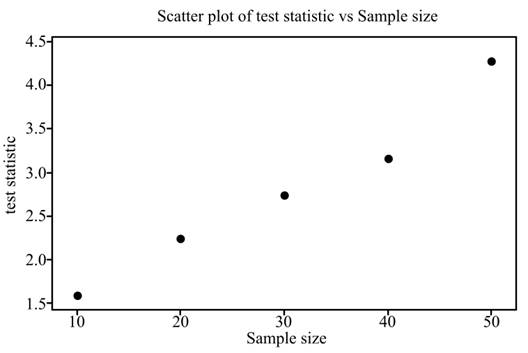
To graph: The values of test statistic versus sample size using the results of sections (1), (2), (3), (4) and (5).
Section 6
Explanation of Solution
Graph: From the results of section 1 to 5, create a table for Sample size and test statistic.
Sample size |
Test statistic |
10 |
1.58 |
20 |
2.24 |
30 |
2.74 |
40 |
3.16 |
50 |
3.54 |
To plot the graph, follow the below mentioned steps in Minitab;
Step1: Enter the data of table in Minitab. Enter variable name as Sample size and test statistic.
Step 2: Go to
Step 3: In the dialog box select ‘simple’ then click Ok.
Step 4: In the new dialog box, enter ‘Test statistic’ as ‘Y variables’ ‘Sample size’ as ‘X variables’. Finally, click OK.
From the Minitab results, the graph is as follows,
Section 7:
To graph: The values of p-test versus sample size using the results of sections (1), (2), (3), (4), and (5).
Section 7:
Explanation of Solution
Graph: From the results of section 1 to 5, create a table for Sample size and test statistic.
Sample size |
p-value |
10 |
0.057 |
20 |
0.013 |
30 |
0.003 |
40 |
0.001 |
50 |
0.000 |
To plot the graph, follow the below mentioned steps in Minitab;
Step1: Enter the data of table in Minitab. Enter variable name as Sample size and p-value.
Step 2: Go to
Step 3: In the dialog box select ‘simple’ then click Ok.
Step 4: In the new dialog box, enter ‘p-value’ under the field marked as ‘Y variables’ ‘Sample size’ under the field marked as ‘X variable’. Finally, click OK.
From the Minitab results, the graph is as follows,
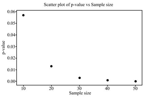
To explain: The effect of the increment in sample size on test statistic and p- value.
Answer to Problem 130E
Solution: As the sample size increases, the value of test statistic increases and the p- value decrease.
Explanation of Solution
Want to see more full solutions like this?
Chapter 6 Solutions
Introduction to the Practice of Statistics


 MATLAB: An Introduction with ApplicationsStatisticsISBN:9781119256830Author:Amos GilatPublisher:John Wiley & Sons Inc
 Probability and Statistics for Engineering and th...StatisticsISBN:9781305251809Author:Jay L. DevorePublisher:Cengage Learning
 Statistics for The Behavioral Sciences (MindTap C...StatisticsISBN:9781305504912Author:Frederick J Gravetter, Larry B. WallnauPublisher:Cengage Learning
 Elementary Statistics: Picturing the World (7th E...StatisticsISBN:9780134683416Author:Ron Larson, Betsy FarberPublisher:PEARSON
 The Basic Practice of StatisticsStatisticsISBN:9781319042578Author:David S. Moore, William I. Notz, Michael A. FlignerPublisher:W. H. Freeman
 Introduction to the Practice of StatisticsStatisticsISBN:9781319013387Author:David S. Moore, George P. McCabe, Bruce A. CraigPublisher:W. H. Freeman