Pearson eText for Statistical Reasoning for Everyday Life -- Instant Access (Pearson+)
5th Edition
ISBN: 9780137561544
Author: Jeffrey Bennett, William Briggs
Publisher: PEARSON+
expand_more
expand_more
format_list_bulleted
Concept explainers
Videos
Textbook Question
Chapter 7, Problem 6CRE
Pizza and the Subway. For Exercises 1–6, refer to the following table that lists the cost (in dollars) of a slice of pizza in New York City and the subway fare in the same year.
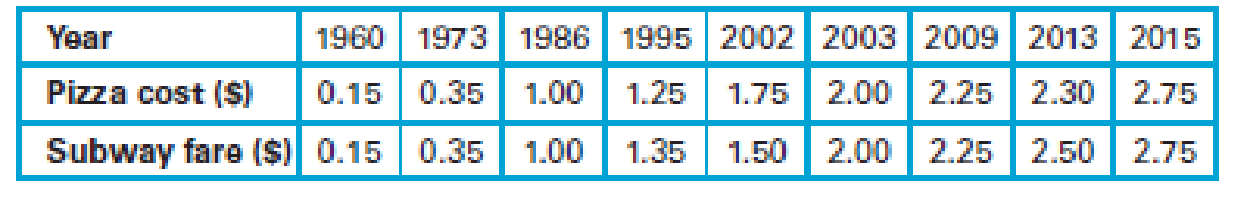
6. Using the equation for the best-fit line, we find that when a slice of pizza costs $1000, the predicted subway fare is $1011. Is that predicted subway fare likely to be an accurate prediction? Why or why not?
Expert Solution & Answer
Want to see the full answer?
Check out a sample textbook solution
Students have asked these similar questions
Complete Part D
A recent issue of the AARP Bulletin reported that the average weekly pay for a woman with a high school degree is $520 (AARP Bulletin, January–February, 2010). Suppose you would like to determine if the average weekly pay for all working women is significantly greater than that for women with a high school degree. Data providing the weekly pay for a sample of 50 working women are available in the file named WeeklyPay. These data are consistent with the findings reported in the AARP article. Complete D
null hyposthesis: H(o)=520Alternative hypothesis: H(a): greater then 520
sample mean=637.94
the test statistic = 5.62
p-value=0.00
Using a=.05, we would reject the null hypothesis.
D. Repeat the hypothesis test using the critical value approach.
582
333
759
633
629
523
320
685
599
753
553
641
290
800
696
627
679
667
542
619
950
614
548
570
678
697
750
569…
Q1. The table provided gives data on indexes of output per hour (X) and real compensation per hour (Y) for the business and nonfarm business sectors of the U.S. economy for 1960–2005. The base year of the indexes is 1992 = 100 and the indexes are seasonally adjusted.
a. Plot Y against X for the two sectors separately.
b. What is the economic theory behind the relationship between the two variables? Does the scattergram support the theory?
c. Estimate the OLS regression of Y on X.
Note: on the table ( 1. Output refers to real gross domestic product in the sector. 2. Wages and salaries of employees plus employers’ contributions for social insurance and private benefit plans. 3. Hourly compensation divided by the consumer price index for all urban consumers for recent quarters.)
Thank you!
Q. Table provided gives data on gross domestic product (GDP) for the United States for the years 1959–2005.
a. Plot the GDP data in current and constant (i.e., 2000) dollars against time.
b. Letting Y denote GDP and X time (measured chronologically starting with 1 for 1959, 2 for 1960, through 47 for 2005), see if the following model fits the GDP data:
Yt = β1 + β2 Xt + ut
Estimate this model for both current and constant-dollar GDP.
c. How would you interpret β2?
d. If there is a difference between β2 estimated for current-dollar GDP and that estimated for constant-dollar GDP, what explains the difference?
e. From your results what can you say about the nature of inflation in the United States over the sample period?
Chapter 7 Solutions
Pearson eText for Statistical Reasoning for Everyday Life -- Instant Access (Pearson+)
Ch. 7.1 - Correlation. What is a correlation? Give three...Ch. 7.1 - Scatterplot. What is a scatterplot, and how is one...Ch. 7.1 - Types of Correlation. Define and distinguish...Ch. 7.1 - Correlation Coefficient. What does the correlation...Ch. 7.1 - Does It Make Sense? For Exercises 58, determine...Ch. 7.1 - Does It Make Sense? For Exercises 58, determine...Ch. 7.1 - Does It Make Sense? For Exercises 58, determine...Ch. 7.1 - Does It Make Sense? For Exercises 58, determine...Ch. 7.1 - Correlation. Exercises 916 list pairs of...Ch. 7.1 - Correlation. Exercises 916 list pairs of...
Ch. 7.1 - Correlation. Exercises 916 list pairs of...Ch. 7.1 - Correlation. Exercises 916 list pairs of...Ch. 7.1 - Correlation. Exercises 916 list pairs of...Ch. 7.1 - Correlation. Exercises 916 list pairs of...Ch. 7.1 - Correlation. Exercises 916 list pairs of...Ch. 7.1 - Correlation. Exercises 916 list pairs of...Ch. 7.1 - Crickets and Temperature. One classic example of a...Ch. 7.1 - Two-Day Forecast. Figure 7.8 shows a scatterplot...Ch. 7.1 - Properties of the Correlation Coefficient. For...Ch. 7.1 - Properties of the Correlation Coefficient. For...Ch. 7.1 - Properties of the Correlation Coefficient. For...Ch. 7.1 - Properties of the Correlation Coefficient. For...Ch. 7.1 - Scatterplot and Correlation. In Exercises 2330,...Ch. 7.1 - Scatterplot and Correlation. In Exercises 2330,...Ch. 7.1 - Scatterplot and Correlation. In Exercises 2330,...Ch. 7.1 - Prob. 26ECh. 7.1 - Scatterplot and Correlation. In Exercises 2330,...Ch. 7.1 - Scatterplot and Correlation. In Exercises 2330,...Ch. 7.1 - Scatterplot and Correlation. In Exercises 2330,...Ch. 7.1 - Scatterplot and Correlation. In Exercises 2330,...Ch. 7.1 - Your Own Positive Correlations. Give examples of...Ch. 7.1 - Your Own Negative Correlations. Give examples of...Ch. 7.2 - Outliers. Briefly explain how an outlier can make...Ch. 7.2 - Grouped Data. Briefly explain how data that...Ch. 7.2 - Explanations for Correlation. What are the three...Ch. 7.2 - Prob. 4ECh. 7.2 - Does It Make Sense? For Exercises 58, determine...Ch. 7.2 - Does It Make Sense? For Exercises 58, determine...Ch. 7.2 - Does It Make Sense? For Exercises 58, determine...Ch. 7.2 - Does It Make Sense? For Exercises 58, determine...Ch. 7.2 - Correlation and Causality. Exercises 916 present...Ch. 7.2 - Correlation and Causality. Exercises 916 present...Ch. 7.2 - Correlation and Causality. Exercises 916 present...Ch. 7.2 - Correlation and Causality. Exercises 916 present...Ch. 7.2 - Correlation and Causality. Exercises 916 present...Ch. 7.2 - Correlation and Causality. Exercises 916 present...Ch. 7.2 - Correlation and Causality. Exercises 916 present...Ch. 7.2 - Correlation and Causality. Exercises 916 present...Ch. 7.2 - Outlier Effects. Consider the scatterplot in...Ch. 7.2 - Outlier Effects. Consider the scatterplot in...Ch. 7.2 - Footprint and Height. The following table lists...Ch. 7.2 - January and July High Temperatures. The following...Ch. 7.2 - Birth and Death Rates. Figure 7.17 shows the birth...Ch. 7.2 - Penny Weight and Date. The scatterplot in Figure...Ch. 7.3 - Best-Fit Line. What is a best-fit line? How is a...Ch. 7.3 - Prob. 2ECh. 7.3 - Interpreting r2. What does the square of the...Ch. 7.3 - Prob. 4ECh. 7.3 - Prob. 5ECh. 7.3 - Does It Make Sense? For Exercises 58, determine...Ch. 7.3 - Does It Make Sense? For Exercises 58, determine...Ch. 7.3 - Does It Make Sense? For Exercises 58, determine...Ch. 7.3 - Best-Fit Lines. Exercises 916 refer to tables in...Ch. 7.3 - Best-Fit Lines. Exercises 916 refer to tables in...Ch. 7.3 - Prob. 11ECh. 7.3 - Best-Fit Lines. Exercises 916 refer to tables in...Ch. 7.3 - Best-Fit Lines. Exercises 916 refer to tables in...Ch. 7.3 - Best-Fit Lines. Exercises 916 refer to tables in...Ch. 7.3 - Prob. 15ECh. 7.3 - Prob. 16ECh. 7.4 - Correlation and Causality. What is the difference...Ch. 7.4 - Prob. 2ECh. 7.4 - Establishing Causality. Briefly state in your own...Ch. 7.4 - Confidence in Causality. Describe three levels of...Ch. 7.4 - Prob. 5ECh. 7.4 - Does It Make Sense? For Exercises 58, determine...Ch. 7.4 - Does It Make Sense? For Exercises 58, determine...Ch. 7.4 - Does It Make Sense? For Exercises 58, determine...Ch. 7.4 - Physical Models. For Exercises 912, determine...Ch. 7.4 - Physical Models. For Exercises 912, determine...Ch. 7.4 - Physical Models. For Exercises 912, determine...Ch. 7.4 - Physical Models. For Exercises 912, determine...Ch. 7.4 - Altitude and Health. When some people climb to...Ch. 7.4 - Smoking and Lung Cancer. There is a strong...Ch. 7.4 - Other Lung Cancer Causes. Several things besides...Ch. 7.4 - Longevity of Orchestra Conductors. A famous study...Ch. 7.4 - Older Moms. A study reported in Nature claims that...Ch. 7.4 - High-Voltage Power Lines. Suppose that people...Ch. 7.4 - Gun Control. Those who favor gun control often...Ch. 7.4 - Vasectomies and Prostate Cancer. The article Does...Ch. 7 - Pizza and the Subway. For Exercises 16, refer to...Ch. 7 - Pizza and the Subway. For Exercises 16, refer to...Ch. 7 - Pizza and the Subway. For Exercises 16, refer to...Ch. 7 - Pizza and the Subway. For Exercises 16, refer to...Ch. 7 - Pizza and the Subway. For Exercises 16, refer to...Ch. 7 - Pizza and the Subway. For Exercises 16, refer to...Ch. 7 - For 10 pairs of sample data values, the...Ch. 7 - In a study involving randomly selected subjects,...Ch. 7 - A researcher collects paired sample data values...Ch. 7 - Estimate the value of the linear correlation...Ch. 7 - Fill in the blanks: Every possible correlation...Ch. 7 - Which of the following are likely to have a...Ch. 7 - For a collection of 50 pairs of sample data...Ch. 7 - Estimate the correlation coefficient for the data...Ch. 7 - Refer again to the scatterplot in Figure 7.24....Ch. 7 - Fill in the blank: If r = 0.900, then _____ % of...Ch. 7 - In Exercises 710, determine whether the given...Ch. 7 - Prob. 8CQCh. 7 - Prob. 9CQCh. 7 - Prob. 10CQ
Knowledge Booster


Learn more about
Need a deep-dive on the concept behind this application? Look no further. Learn more about this topic, statistics and related others by exploring similar questions and additional content below.Similar questions
- section 4.1 #30 In Exercises 25–30, determine whether the association between the two variables is positive or negative. Weekly ice cream sales and weekly average temperaturearrow_forwardIn 2010, MonsterCollege surveyed 1250 U.S.college students expecting to graduate in the next several years.Respondents were asked the following question:What do you think your starting salary will be at your firstjob after college?The line graph shows the percentage of college students whoanticipated various starting salaries. Use the graph to solveExercises 9–14. What starting salary was anticipated by the greatestpercentage of college students? Estimate the percentage ofstudents who anticipated this salary? What starting salary was anticipated by the least percentageof college students? Estimate the percentage of students whoanticipated this salary? What starting salaries were anticipated by more than 20% ofcollege students? Estimate the percentage of students who anticipated astarting salary of $40 thousand.arrow_forwardWorld Military Expenditure The following chart shows total military and arms trade expenditure from 2011–2020 (t = 1 represents 2011). †A bar graph titled "World military expenditure" has a horizontal t-axis labeled "Year since 2010" and a vertical axis labeled "$ (billions)". The bar graph has 10 bars. Each bar is associated with a label and an approximate value as listed below. 1: 1,800 billion dollars 2: 1,775 billion dollars 3: 1,750 billion dollars 4: 1,730 billion dollars 5: 1,760 billion dollars 6: 1,760 billion dollars 7: 1,850 billion dollars 8: 1,900 billion dollars 9: 1,950 billion dollars 10: 1,980 billion dollars (a) If you want to model the expenditure figures with a function of the form f(t) = at2 + bt + c, would you expect the coefficient a to be positive or negative? Why? HINT [See "Features of a Parabola" in this section.] We would expect the coefficient to be positive because the curve is concave up. We would expect the coefficient to be negative because the…arrow_forward
- The figure shows the graphs of the cost and revenue functions for a company that manufactures and sells small radios. Use the information in the figure to solve Exercises 67–72. 35,000 30,000 C(x) = 10,000 + 30x 25,000 20,000 15,000 R(x) = 50x 10,000 5000 100 200 300 400 500 600 700 Radios Produced and Sold 67. How many radios must be produced and sold for the company to break even? 68. More than how many radios must be produced and sold for the company to have a profit? 69. Use the formulas shown in the voice balloons to find R(200) – C(200). Describe what this means for the company. 70. Use the formulas shown in the voice balloons to find R(300) – C(300). Describe what this means for the company. 71. a. Use the formulas shown in the voice balloons to write the company's profit function, P, from producing and selling x radios. b. Find the company's profit if 10,000 radios are produced and sold. 72. a. Use the formulas shown in the voice balloons to write the company's profit function,…arrow_forwardQ. Table gives data on gold prices, the Consumer Price Index (CPI), and the New York Stock Exchange (NYSE) Index for the United States for the period 1974 –2006. The NYSE Index includes most of the stocks listed on the NYSE, some 1500-plus. a. Plot in the same scattergram gold prices, CPI, and the NYSE Index. b. An investment is supposed to be a hedge against inflation if its price and /or rate of return at least keeps pace with inflation. To test this hypothesis, suppose you decide to fit the following model, assuming the scatterplot in (a) suggests that this is appropriate: Gold pricet = β1 + β2 CPIt + ut NYSE indext = β1 + β2 CPIt + ut Note that if beta2 = 1 the response exactly grows with CPI Thank you!arrow_forwardThe table shows the historical in-state tuition rates for the University of Kalamazoo. Use the data to answer the questions and round your answers to two decimal places. Academic year Rate of tuition for one semester 2008–2009 $3,812 2009–2010 $4,002 2010–2011 $4,441 2011–2012 $4,905 2012–2013 $5,181 What is the percentage increase in tuition from the 2008–2009 school year to the 2012–2013 school year?arrow_forward
- Insurance Rates The following table gives themonthly insurance rates for a $100,000 life insurancepolicy for smokers 35–50 years of age.a. Create a scatter plot for the data.b. Does it appear that a quadratic function can beused to model the data? If so, find the best-fittingquadratic model.c. Find the power model that is the best fit for the data.d. Compare the two models by graphing each modelon the same axes with the data points. Whichmodel appears to be the better fit?arrow_forwardExercises 93–94: Energy The following graph shows U.S. Energy consumption. 400 350 300 250 200 150 100 50 04 1970 1990 2010 Year 93. When was energy consumption increasing? 94. When was energy consumption decreasing? Energy (millions of Btu)arrow_forwardU.S. Population The number of White non-Hispanicindividuals in the U.S. civilian non-institutional population 16 years and older was 153.1 million in 2000and is projected to be 169.4 million in 2050.(Source: U.S. Census Bureau)a. Find the average annual rate of change in population during the period 2000–2050, with the appropriate units.b. Use the slope from part (a) and the population in2000 to write the equation of the line associatedwith 2000 and 2050.c. What does this model project the population to bein 2020?arrow_forward
- International Visitors The number of internationalvisitors to the United States for selected years 1986–2010 is given in the table below. If you had to pick one of these models to predictthe number of international visitors in the year2020, which model would be the more reasonablechoice?arrow_forwardRegression and Predictions. Exercises 13–28 use the same data sets as Exercises 13–28 in Section 10-1. In each case, find the regression equation, letting the first variable be the predictor (x) variable. Find the indicated predicted value by following the prediction procedure summarized in Figure 10-5 on page 493. Old Faithful Using the listed duration and interval after times, find the best predicted “interval after” time for an eruption with a duration of 253 seconds. How does it compare to an actual eruption with a duration of 253 seconds and an interval after time of 83 minutes?arrow_forwardPage of 11 ZOOM + 5. The table shows how the cost of a carne asada taco at my favorite taco stand has increased as they have become more popular since their opening in 2013. Use the data to answer the questions below. Year, x 2013, 0 2014, 1 2015, 2 2016, 3 2017, 4 2018, 5 2019,6 Cost ($) 0.50 0.55 0.65 0.75 0.90 1.00 1.10 (a) What is the regression line given by your TI-84 for this data? Round values to 3 decimal places. (b) Using the regression equation above, predict the cost of a carne asada taco at my favorite taco stand in 2020. Show the work.arrow_forward
arrow_back_ios
SEE MORE QUESTIONS
arrow_forward_ios
Recommended textbooks for you
 MATLAB: An Introduction with ApplicationsStatisticsISBN:9781119256830Author:Amos GilatPublisher:John Wiley & Sons Inc
 Probability and Statistics for Engineering and th...StatisticsISBN:9781305251809Author:Jay L. DevorePublisher:Cengage Learning
 Statistics for The Behavioral Sciences (MindTap C...StatisticsISBN:9781305504912Author:Frederick J Gravetter, Larry B. WallnauPublisher:Cengage Learning
 Elementary Statistics: Picturing the World (7th E...StatisticsISBN:9780134683416Author:Ron Larson, Betsy FarberPublisher:PEARSON
 The Basic Practice of StatisticsStatisticsISBN:9781319042578Author:David S. Moore, William I. Notz, Michael A. FlignerPublisher:W. H. Freeman
 Introduction to the Practice of StatisticsStatisticsISBN:9781319013387Author:David S. Moore, George P. McCabe, Bruce A. CraigPublisher:W. H. Freeman
MATLAB: An Introduction with Applications
Statistics
ISBN:9781119256830
Author:Amos Gilat
Publisher:John Wiley & Sons Inc
Probability and Statistics for Engineering and th...
Statistics
ISBN:9781305251809
Author:Jay L. Devore
Publisher:Cengage Learning
Statistics for The Behavioral Sciences (MindTap C...
Statistics
ISBN:9781305504912
Author:Frederick J Gravetter, Larry B. Wallnau
Publisher:Cengage Learning
Elementary Statistics: Picturing the World (7th E...
Statistics
ISBN:9780134683416
Author:Ron Larson, Betsy Farber
Publisher:PEARSON
The Basic Practice of Statistics
Statistics
ISBN:9781319042578
Author:David S. Moore, William I. Notz, Michael A. Fligner
Publisher:W. H. Freeman
Introduction to the Practice of Statistics
Statistics
ISBN:9781319013387
Author:David S. Moore, George P. McCabe, Bruce A. Craig
Publisher:W. H. Freeman
Use of ALGEBRA in REAL LIFE; Author: Fast and Easy Maths !;https://www.youtube.com/watch?v=9_PbWFpvkDc;License: Standard YouTube License, CC-BY
Compound Interest Formula Explained, Investment, Monthly & Continuously, Word Problems, Algebra; Author: The Organic Chemistry Tutor;https://www.youtube.com/watch?v=P182Abv3fOk;License: Standard YouTube License, CC-BY
Applications of Algebra (Digit, Age, Work, Clock, Mixture and Rate Problems); Author: EngineerProf PH;https://www.youtube.com/watch?v=Y8aJ_wYCS2g;License: Standard YouTube License, CC-BY