
Concept explainers
Videos
(a)
Section 1:
To find: The difference between the TBBMC recorded for Operator 1 and the TBBMC for Operator 2.
(a)
Section 1:
Answer to Problem 43E
Solution: The table for difference is as follows:
Operator 1 |
Operator 2 |
Difference |
1.328 |
1.323 |
0.005 |
1.342 |
1.322 |
0.02 |
1.075 |
1.073 |
0.002 |
1.228 |
1.233 |
−0.005 |
0.939 |
0.934 |
0.005 |
1.004 |
1.019 |
−0.015 |
1.178 |
1.184 |
−0.006 |
1.286 |
1.304 |
−0.018 |
Explanation of Solution
Calculation:
To calculate the difference, follow the below mentioned steps in Minitab:
Step 1: Enter the variable name as “Operator 1” in column C1 and enter the data for “Operator 1” and enter the variable name as “Operator 2” in column C2 and enter the data for “Operator 2.”
Step 2: Enter variable name as “Difference” in column C3.
Step 3: Go to
Step 4: In the dialog box that appears, select “Difference” in “Store result in variable.”
Step 5: Enter “Operator 1”-“Operator 2” in “Expression.” Click on “Ok” on the dialog box.
From Minitab result, the table for difference is as follows:
Operator 1 |
Operator 2 |
Difference |
1.328 |
1.323 |
0.005 |
1.342 |
1.322 |
0.02 |
1.075 |
1.073 |
0.002 |
1.228 |
1.233 |
−0.005 |
0.939 |
0.934 |
0.005 |
1.004 |
1.019 |
−0.015 |
1.178 |
1.184 |
−0.006 |
1.286 |
1.304 |
−0.018 |
Interpretation: It is clear from the table that the
Section 2:
To test: Whether t- methods can be used or not.
Section 2:
Answer to Problem 43E
Solution: The t- method can be used.
Explanation of Solution
Calculation:
To determine if the t methods can be used or not, a probability plot is drawn in Minitab by following the below mentioned steps:
Step 1: Follow steps 1 and 2 similar to that in Section 1.
Step 2: Go to “Graph” option and click on “Probability Plot.” In the dialog box that appears, select “Single” and click on OK.
Step 3: Then enter the name of the column containing the data of the differences in the “Graph variables” field and click on OK.
The following probability plot is obtained:
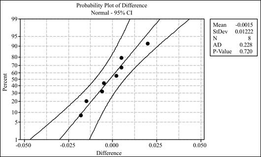
Conclusion: The probability plot shows that the data is approximately normal as all the data points fall within the range and, hence, it is appropriate to use t procedures.
(b)
To test: The significance of the difference between the means of two operators.
(b)
Answer to Problem 43E
Solution: The test statistic value is
Explanation of Solution
Calculation:
To test the null hypothesis, follow the below mentioned steps in Minitab:
Step 1: Follow the Steps 1 to 5 performed in section 1 of part (a).
Step 2: Go to
Step 3: In the dialogue box that appears, select samples in columns.
Step 4: Enter “Operator 1” under the field marked as “First sample” and “Operator 2” under the field marked as “Second sample.”
Step 5: In the dialogue box that appears, Click on “Option.” Enter 95.0 in the field of Confidence interval, 0.0 in “Test mean,” and “not equal” in “Alternative.”
From Minitab results, the value of test statistic is
D.F = n –.
D.F = 8 –.
D.F =.
Conclusion: If the level of significance is 5% then as the p- value is greater than 0.05 the null hypothesis will not be rejected and it is concluded that the two means do not differ significantly at 95% confidence level.
(c)
To find: The confidence interval for difference.
(c)
Answer to Problem 43E
Solution: The required confidence interval is
Explanation of Solution
Calculation: To compute the confidence interval, follow the below mentioned steps in Minitab:
Step 1: Follow the steps 1 to 5 performed in section 1 of part (a).
Step 2: Go to
Step 3: In the dialogue box that appears, select samples in columns.
Step 4: Enter “Operator 1” under the field marked as “First sample” and “Operator 2” under the field marked as “Second sample.”
Step 5: In the dialogue box that appears, Click on “Option.” Enter 95.0 in the field of Confidence interval, 0.0 in “Test mean,” and “not equal” in “Alternative.”
From the Minitab results, the confidence interval is
Interpretation: The confidence interval denotes that the differences recorded will lie in between −0.01172 and 0.00872 with a possible chance of 5% error.
(d)
The validity of the results if the samples are not random.
(d)
Answer to Problem 43E
Solution: The testing results and the confidence interval may not be valid if the samples are non-random.
Explanation of Solution
Want to see more full solutions like this?
Chapter 7 Solutions
INTRO.TO PRACTICE STATISTICS-ACCESS


 MATLAB: An Introduction with ApplicationsStatisticsISBN:9781119256830Author:Amos GilatPublisher:John Wiley & Sons Inc
 Probability and Statistics for Engineering and th...StatisticsISBN:9781305251809Author:Jay L. DevorePublisher:Cengage Learning
 Statistics for The Behavioral Sciences (MindTap C...StatisticsISBN:9781305504912Author:Frederick J Gravetter, Larry B. WallnauPublisher:Cengage Learning
 Elementary Statistics: Picturing the World (7th E...StatisticsISBN:9780134683416Author:Ron Larson, Betsy FarberPublisher:PEARSON
 The Basic Practice of StatisticsStatisticsISBN:9781319042578Author:David S. Moore, William I. Notz, Michael A. FlignerPublisher:W. H. Freeman
 Introduction to the Practice of StatisticsStatisticsISBN:9781319013387Author:David S. Moore, George P. McCabe, Bruce A. CraigPublisher:W. H. Freeman