Concept explainers
Videos
In 1990, the population of the African country Benin was about 4.6 million people. Its composition by age was as follows:
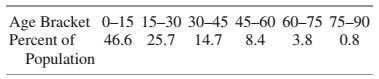
We represent these data in a state
We measure time in increments of 15 years, with
a. Explain the significance of all the entries in the matrix A in terms of population dynamics.
b. Find the eigenvalue of A with the largest modulus and an associated eigenvector (use technology).What is the significance of these quantities in terms of population dynamics? (For a summary on matrix techniques used in the study of age-structured populations, see Dmitrii O. Logofet, Matrices andGraphs: Stability Problems in Mathematical Ecology, Chapters 2 and 3, CRC Press, 1993.)
Want to see the full answer?
Check out a sample textbook solution
Chapter 7 Solutions
Linear Algebra with Applications (2-Download)


- The following Minitab display gives information regarding the relationship between the body weight of a child (in kilograms) and the metabolic rate of the child (in 100 kcal/ 24 hr). Predictor Coef SE Coef T PConstant 0.8570 0.4148 2.06 0.84Weight 0.38243 0.02978 13.52 0.000 S = 0.517508 R-Sq = 97.4% (a) Write out the least-squares equation. y^= ______ + _____x (b) For each 1 kilogram increase in weight, how much does the metabolic rate of a child increase? (Use 5 decimal places.)arrow_forwardUse this data and create a model that estimates a student's giving rate as an alumni based on the three parameters provided. If a class has a graduation rate of 74, the % of classes under 20 student equal to 55, and a Student=Faculty Ratio of 19, what should we expect our Alumni Giving Rate to be? (Enter a whole number) University Graduation Rate % of Classes Under 20 Student-Faculty Ratio Alumni Giving Rate Boston College 85 39 13 25 Brandeis University 79 68 8 33 Brown University 93 60 8 40 California Institute of Technology 85 65 3 46 Carnegie Mellon University 75 67 10 28 Case Western Reserve Univ. 72 52 8 31 College of William and Mary 89 45 12 27 Columbia University 90 69 7 31 Cornell University 91 72 13 35 Dartmouth College 94 61 10 53 Duke University 92 68 8 45 Emory University 84 65 7 37 Georgetown University 91 54 10 29 Harvard University 97 73 8 46 Johns Hopkins University 89 64 9 27 Lehigh University 81 55 11 40 Massachusetts Inst.…arrow_forwardFind the least-squares equation for the following pairs of data: x = earthquake magnitude 2.9 4.2 3.3 4.5 2.6 3.2 3.4 y = depth of earthquake (in km) 5 10 11.2 10 7.9 3.9 5.5 A. y = 2.16 + 0.221x B. y = 0.221 + 2.16x C. y = 2.16 + 0.312x D. y = 0.221 + 2.82xarrow_forward
- The following table gives the millions of metric tons of carbon dioxide emissions in a certain country for selected years from 2010 and projected to 2032. Year 2010 2012 2014 2016 2018 2020 CO2 Emissions 337.5 361.5 395.1 425.8 451.1 496.4 Year 2022 2024 2026 2028 2030 2032 CO2 Emissions 558.2 592.9 628.7 662.1 709.1 742.7 (a) Create a linear function that models these data, with x as the number of years past 2010 and y as the millions of metric tons of carbon dioxide emissions. (Round all numerical values to two decimal places.)y(x) = (b) Find the model's estimate for the 2028 data point. (Round your answer to two decimal places.) million metric tons(c) Find the slope of the linear model. (Round your answer to two decimal places.)Interpret the slope of the linear model. For each year since ---Select--- 2009 2010 2015 2028 2032 , carbon dioxide emissions in the U.S. are expected to change by million metric tons.arrow_forwardNeed help with parts d and k. Data: TSERofReturn AcmeRofReturn 1 0.42478 -0.48194 2 1.61213 -0.73284 3 -0.98754 -2.28445 4 -0.30013 -1.55312 5 1.41215 0.68674 6 0.68725 -1.31132 7 0.03733 -0.83295 8 -1.72494 -1.71975 9 0.33729 1.14443 10 -1.07502 -1.79885 11 0.86222 0.89736 12 1.17468 1.66664 13 -0.38761 -0.02658 14 1.66212 0.9086 15 1.09969 1.99935 16 -0.06266 0.46148 17 -1.96241 -1.41004 18 -1.32499 -0.38086 19 -1.51247 -1.90904 20 0.74974 0.91873 21 -0.38761 -0.49714 22 -0.17514 -1.31385 23 -3.41222 -1.15681 24 -0.01266 2.11718 25 0.16231 1.78766 26 -0.82506 1.30344 27 -0.41261 -0.43377 28 0.2623 -1.70274 29 -1.16251 0.4692 30 -1.05003 0.27671 31 -0.65008 -0.63741 32 0.62475 2.9895 33 -0.68758 1.3613 34…arrow_forwardThe table below contains the average public school classroom teacher's salaries, S, for an 11-year period. Letting t=0 represent 1990,t=1 for 1991 and so on, use a graphing utility to find a linear model for the data. Year 1990 1991 1992 1993 1994 1995 Salary 33099 32478 34024 37111 37541 36684 Year 1996 1997 1998 1999 2000 Salary 37803 38055 39327 43052 42163 Salary, written as a function of t is given by S(t)=arrow_forward
- The table contains data on vehicle speed (h) and fuel consumption (lt / 100km) of 5 randomly selected vehicles. Estimate the average fuel consumption of a vehicle traveling at 45 km / h using the simple linear regression equation between vehicle speed and fuel consumption. Speed 55 60 65 70 75 Consumption 13 12 11 10 9 a. 15 b. 8 c. 7 d. 20arrow_forwardYou have the following data: Gasoline Sales during 2017.1 to 2020.4 (in 000 of barrels) Year and quarter Gasoline Sales Year and quarter Gasoline sales 2017.1 22434 2019.1 22776 2017.2 23766 2019.2 24491 2017.3 23860 2019.3 24751 2017.4 23391 2019.4 24170 2018.1 22662 2020.1 23302 2018.2 24032 2020.2 24045 2018.3 24171 2020.3 25437 2018.4 23803 2020.4 25272 (A)Using data on gasoline sales (in thousands of barrels) from the first quarter of 2017 to the last quarter of 2020, estimate the secular linear trend equation. (B) Accordingly, forecast gasoline sales for the four quarters of 2021. (C)Use the dummy variables methods to adjust the trend forecasts for the four quarters of2021 you made in (B) above to take the seasonal…arrow_forwardThe following data gives U. S. population in millions in the indicated year. Year US population (in millions) 1960 180.7 1970 205.1 1980 227.7 1990 249.9 2000 281.4 2010 308.7 Determine the linear regression model. Again t=0 in 1960.arrow_forward
- Consider the following log-wage regression results for women (W) and men (M) where wages are predicted by schooling (S) and age (A). wW = 2.23 + 0.077Sw + 0.017Aw and wM = 2.33 + 0.0745SM + 0.026AM. Sample means for the variables by gender are: women average a logged wage of 3.90, 12.7 years of schooling, and 40.8 years-old; men average a logged wage of 4.53, 14.2 years of schooling, and 43.9 years-old. Decompose the raw difference in average logged wages using the Oaxaca-Blinder decomposition. Specifically, decompose the raw difference into the portion due to differences in schooling, differences in age, and the portion left unexplained, possibly due to gender discrimination.arrow_forwardConsider the following model constructed by researchers investigating the relationship between blood pressure and BMI, controlling for age:BMI=α+ β1*(Systolic blood pressure)+β2*(Age) A) Describe the interpretation of each of the following: α, β1, β2. How many dimensions are being observed in the response surface depicted by this model?arrow_forwardShow that the functions e^x , e^2x , e^3x are linearly independent.arrow_forward
 Algebra and Trigonometry (6th Edition)AlgebraISBN:9780134463216Author:Robert F. BlitzerPublisher:PEARSON
 Contemporary Abstract AlgebraAlgebraISBN:9781305657960Author:Joseph GallianPublisher:Cengage Learning
 Linear Algebra: A Modern IntroductionAlgebraISBN:9781285463247Author:David PoolePublisher:Cengage Learning
 Algebra And Trigonometry (11th Edition)AlgebraISBN:9780135163078Author:Michael SullivanPublisher:PEARSON
 Introduction to Linear Algebra, Fifth EditionAlgebraISBN:9780980232776Author:Gilbert StrangPublisher:Wellesley-Cambridge Press
 College Algebra (Collegiate Math)AlgebraISBN:9780077836344Author:Julie Miller, Donna GerkenPublisher:McGraw-Hill Education