Videos
Determining the velocity of particles settling through fluids is of great importance of many areas of engineering and science. Such calculations depend on the flow regime as represented by the dimensionless Reynolds number,
where
where
where
(a) Combine Eqs. (P8.48.2), (P8.48.3), and (P8.48.4) to express the determination of v as a roots of equations problem. That is, express the combined formula in the format
(b) Use the modified secant method with
(c) Based on the result of (b), compute the Reynolds number and the drag coefficient, and use the latter to confirm that the flow regime is not laminar.
(d) Develop a fixed-point iteration solution for the conditions outlined in (b).
(e) Use a graphical approach to illustrate that the formulation developed in (d) will converge for any positive guess.
(a)
To calculate: The equation for the velocity of the particles that settle inside fluids in the form
Answer to Problem 48P
Solution: The desired equation for the velocity of the settling particles is
Explanation of Solution
Given Information:
The relation between the fluid’s velocity in
Here, d is the diameter of the object in m,
Formula Used:
When the Reynolds number is less than 0.1, the Stokes law states that:
Here, g is the gravitational constant and
When the Reynolds number is higher,
Here
Calculation:
Consider the formula for the Reynolds’ number:
Substitute the value of the Reynolds number in the formula for the drag coefficient.
Now replace the value of the drag coefficient from equation
Now create a function whose zero is same as the root of this equation:
This is the desired equation.
(b)
To calculate: The zero of the function obtained in part (a) using the modified secant method where
Answer to Problem 48P
Solution: The velocity of the iron particle settling in water is
Explanation of Solution
Given Information:
The diameter of the iron particle is
Formula Used:
The iterative scheme for the modified secant method is of the form:
where
Calculation:
Note that the dimensions of the diameter, particle density, water density, and the viscosity of water are different to what can be used in the equation obtained in part (a).
Convert the dimensions as follows:
And,
And,
And,
The modified secant method requires an initial guess. This can be obtained using Stoke’s law.
Now the modified secant method can be started. This will be done using MATLAB.
Code:
The mod_secant.m file
function
while(
if
end
end
end
The func.m file
function
end
Output:
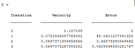
Note that in the third iteration the absolute relative percentage error falls below 0.05%.
Hence the desired velocity can be approximated as
(c)
To calculate: The Reynolds number and the drag coefficient for the iron particles that settle in water and then determine whether the flow in laminar or not.
Answer to Problem 48P
Solution: The Reynolds number is 9.95821429 and the drag coefficient is 3.70074225. This implies that the flow is not laminar.
Explanation of Solution
Given Information:
The velocity of the iron particle settling in water is
Formula Used:
The relation between the fluid’s velocity in
Here, d is the diameter of the object in m,
Calculation:
Substitute 0.0697075 for the v, 0.0002 for d, 1000 for
Hence, the Reynolds number is 9.95821429. As this is greater than 0.1, the flow is non-laminar.
Now substitute 9.95821429 for Re in the formula for the drag-coefficient to obtain:
Thus, the drag coefficient is 3.70074225.
(d)
To calculate: The zero of the function obtained in part (a) using the fixed point method where
Answer to Problem 48P
Solution: The velocity of the iron particle settling in water is
Explanation of Solution
Given Information:
The diameter of the iron particle is
Formula Used:
The iterative scheme for the fixed point method is of the form:
Calculation:
Note that the dimensions of the diameter, particle density, water density, and the viscosity of water are different to what can be used in the equation obtained in part (a).
Convert the dimensions as follows:
And,
And,
And,
The fixed point method requires an initial guess. This can be obtained using Stoke’s law.
Consider the equation whose root needs to obtain as velocity:
Now proceed with the fixed-point method using MATLAB.
Code:
The fixed_point.m file
function
while(
if
end
end
end
The g.m file
function
end
Output:
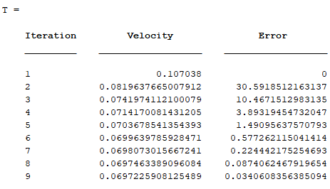
This shows that after the 9th iteration, the approximate relative percentage error reaches below 0.05%.
Hence the desired velocity can be approximated as
(e)
To prove: The function whose root was computed in part (d) would converge using the fixed point iteration irrespective of a positive initial guess.
Explanation of Solution
Given Information:
The diameter of the iron particle is
Formula Used:
The function in terms of the velocity whose zero or root was computed in part (d) was
Proof:
The fixed point iteration for a function
This is iteratively rewritten as:
Use equation
Now graph the functions on the right and on the left of the provided equation.
This can be done using MATLAB.
Code:
Graph:
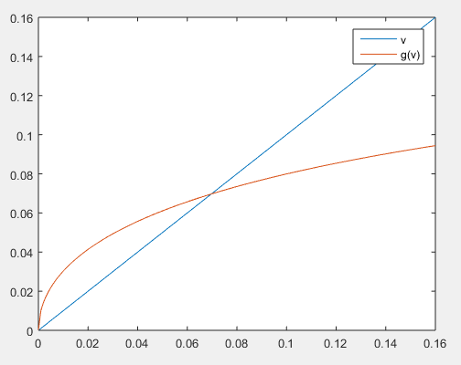
Interpretation:
Note that the graph is divided into two parts. The first part where the function
For both the parts, it is clear that any positive guess say
A line drawn horizontal from
Now proceeding the same way as before, the iterative method would approach the true root. Note that this would occur irrespective of the positive value of
This can be illustrated as:
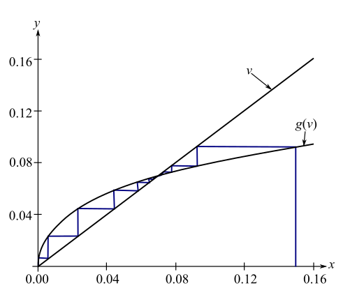
Hence, the fixed point method would converge irrespective of the positive initial guess
Want to see more full solutions like this?
Chapter 8 Solutions
Package: Numerical Methods For Engineers With 2 Semester Connect Access Card
Additional Math Textbook Solutions
Basic Technical Mathematics
Advanced Engineering Mathematics
Fundamentals of Differential Equations (9th Edition)
Glencoe Algebra 2 Student Edition C2014
Linear Algebra with Applications (2-Download)


 Functions and Change: A Modeling Approach to Coll...AlgebraISBN:9781337111348Author:Bruce Crauder, Benny Evans, Alan NoellPublisher:Cengage Learning
 College Algebra (MindTap Course List)AlgebraISBN:9781305652231Author:R. David Gustafson, Jeff HughesPublisher:Cengage Learning