
Videos
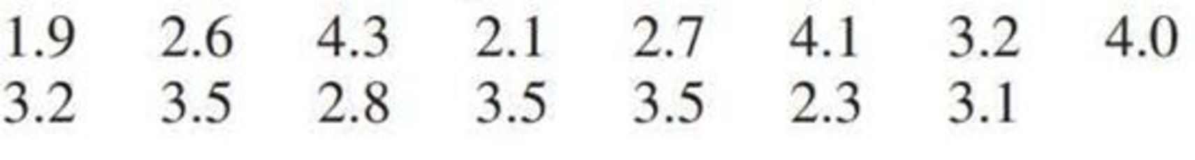
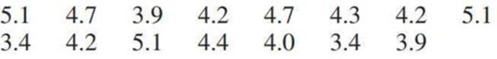
The authors of the paper “Influence of Biofeedback Weight Bearing Training in Sit to Stand to Sit and the Limits of Stability on Stroke Patients” (The Journal of Physical Therapy Science [2016]: 3011–2014) randomly selected two samples of patients admitted to the hospital after suffering a stroke. One sample was selected from patients who received biofeedback weight training for 8 weeks and the other sample was selected from patients who did not receive this training. At the end of 8 weeks, the time it took (in seconds) to stand from a sitting position and then to sit down again (called sit-stand-sit time) was measured for the people in each sample. Data consistent with summary quantities given in the paper are given below. For purposes of this exercise, you can assume that the samples are representative of the population of stroke patients who receive the biofeedback training and the population of stroke patients who do not receive this training.
Biofeedback Group
No Biofeedback Group
- a. Use the given data to estimate the
mean sit-stand-sit time for stroke patients who receive biofeedback training. - b. Use the given data to estimate the mean sit-stand-sit time for stroke patients who do not receive biofeedback training.
- c. Use the given information to estimate the standard deviation of sit-stand-sit times for stroke patients who receive biofeedback.
Want to see the full answer?
Check out a sample textbook solution
Chapter 9 Solutions
INTRODUCTION TO STATISTICS & DATA ANALYS


- A large manufacturing company investigated the service it received from its suppliers and discovered that, in the past, 38% of all material shipments were received late. However, the company recently installed a just-in-time system in which suppliers are linked more closely to the manufacturing process. A random sample of 150 deliveries since the just-in-time system was installed reveals that 33 deliveries were late. If we want to test whether the proportion of late deliveries was reduced signicantly at = 0:10 the null and alternative hypotheses are a. Null hypothesis (H0) b. Alternative hypothesis (HA)arrow_forwardThe researchers reported:" A 2x2 ANOVA revealed, first of all, a main effect for depletion, indicating that depleted individuals generated less ideas (M = 9.40, SD = 5.64) than non-depleted individuals (M = 12.44, SD = 7.34), F (1, 108) = 6.03, p = .016, n2 = .05. This effect was qualified by the expected interaction with [perseverance], F (1,108) = 4.52, p = .036, n2 = .05". What size are the effects for the main effect of depletion and for the interaction between depletion and perseverance, according to Cohen's conventions? a. These are small- to -medium effects b. These are non existent effects c. These are large effects d. We are unable to tell from from the n2 / r2 statisticsarrow_forwardThe authors of the article “Predictive Model for PittingCorrosion in Buried Oil and Gas Pipelines”(Corrosion, 2009: 332–342) provided the data on whichtheir investigation was based.a. Consider the following sample of 61 observations onmaximum pitting depth (mm) of pipeline specimensburied in clay loam soil. 0.41 0.41 0.41 0.41 0.43 0.43 0.43 0.48 0.480.58 0.79 0.79 0.81 0.81 0.81 0.91 0.94 0.941.02 1.04 1.04 1.17 1.17 1.17 1.17 1.17 1.171.17 1.19 1.19 1.27 1.40 1.40 1.59 1.59 1.601.68 1.91 1.96 1.96 1.96 2.10 2.21 2.31 2.462.49 2.57 2.74 3.10 3.18 3.30 3.58 3.58 4.154.75 5.33 7.65 7.70 8.13 10.41 13.44Construct a stem-and-leaf display in which the twolargest values are shown in a last row labeled HI.b. Refer back to (a), and create a histogram based oneight classes with 0 as the lower limit of the firstclass and class widths of .5, .5, .5, .5, 1, 2, 5, and 5,respectively.c. The accompanying comparative boxplot fromMinitab shows plots of pitting depth for four differenttypes of soils.…arrow_forward
- The authors of the article "Adjuvant Radiotherapy and Chemotherapy in Node-Positive Premenopausal Women with Breast Cancer"† reported on the results of an experiment designed to compare treating cancer patients with chemotherapy only to treatment with a combination of chemotherapy and radiation. Of the 154 individuals who received the chemotherapy-only treatment, 76 survived at least 15 years, whereas 98 of the 164 patients who received the hybrid treatment survived at least that long. With p1 denoting the proportion of all such women who, when treated with just chemotherapy, survive at least 15 years and p2 denoting the analogous proportion for the hybrid treatment, p̂1 = (rounded to three decimal places) and p̂2 = (rounded to three decimal places). A confidence interval for the difference between proportions based on the traditional formula with a confidence level of approximately 99% is 0.494 − 0.598 ± (2.58) (0.494)(0.506) 154 + (0.598)(0.402) 164…arrow_forwardA sample of men and women who had passed their driver's test either the first time or the second time were surveyed, with the following results: Results of the driving testGender First time Second timeMen 126 211Women 135 178a) Do these data suggest that there is a relationship between gender and the passing of their driver’s test from which the present sample was drawn? Let alpha=.05arrow_forwardA suburban hotel derives its revenue from its hotel and restaurant operations. Theowners are interested in the relationship between the number of rooms occupied on anightly basis and the revenue per day in the restaurant. Below is a sample of 25 days(Monday through Thursday) from last year showing the restaurant income and numberof rooms occupied.arrow_forward
- A U.S. Food Survey showed that Americans routinely eat beef in their diet. Suppose that in a study of 49 consumers in Illinois and 64 consumers in Texas the following results were obtained from two samples regarding average yearly beef consumption: Illinois Texas = 49 = 64 = 54.1lb = 60.4lb S1 = 7.0 S2 = 8.0 Formulate a hypothesis so that, if the null hypothesis is rejected, we can conclude that the average amount of beef eaten annually by consumers in Illinois is significantly less than that eaten by consumers in Texas.arrow_forward19. A local brewery produces three premium lagers named Half Pint, XXX, and Dark Knight. Of its premium lagers, the brewery bottles 40% Half Pint, 40% XXX, and 20% Dark Knight. In a marketing test of a sample of 80 consumers, 26 preferred the Half Pint lager, 42 preferred the XXX lager, and 12 preferred the Dark Night lager. Using a chi-square goodness-of-fit test, test whether the production of the premium lagers matches these consumer preferences using a .05 level of significance. 19a. Step 2: Compute the df and locate the critical values. df = _______ Critical value = ________arrow_forward19. A local brewery produces three premium lagers named Half Pint, XXX, and Dark Knight. Of its premium lagers, the brewery bottles 40% Half Pint, 40% XXX, and 20% Dark Knight. In a marketing test of a sample of 80 consumers, 26 preferred the Half Pint lager, 42 preferred the XXX lager, and 12 preferred the Dark Night lager. Using a chi-square goodness-of-fit test, test whether the production of the premium lagers matches these consumer preferences using a .05 level of significance. 19. Step 1: Which of the following is the correct set of hypotheses?A. H0: The preferences will not match production (40% Half Pint, 40% XXX, 20% Dark Knight); and H1: The preferences will match production B. H0: \mu_{1}μ1 = \mu_{2}μ2 = \mu_{3}μ3; and H1: At least one of the categories will be different than the others C. H0: The preferences will match production (40% Half Pint, 40% XXX, 20% Dark Knight); and H1: The preferences will not match production 19b. Step 2: Compute the df and locate the…arrow_forward
- 19. A local brewery produces three premium lagers named Half Pint, XXX, and Dark Knight. Of its premium lagers, the brewery bottles 40% Half Pint, 40% XXX, and 20% Dark Knight. In a marketing test of a sample of 80 consumers, 26 preferred the Half Pint lager, 42 preferred the XXX lager, and 12 preferred the Dark Night lager. Using a chi-square goodness-of-fit test, test whether the production of the premium lagers matches these consumer preferences using a .05 level of significance. 19. Step 3: Compute the test statistic -- Chi-square χ2 = (use 2 decimal places) _____________ Step 4: Decision and Conclusions 19. Step 4: Decision: A. Reject H0 B. Retain H0 19. Step 5: Conclusion: Did the production of the premium lagers match consumer preferences? A. Yes. The observed frequencies did not differ from the expected frequencies. B. No. The observed frequencies differed from the expected frequencies.arrow_forward19. A local brewery produces three premium lagers named Half Pint, XXX, and Dark Knight. Of its premium lagers, the brewery bottles 40% Half Pint, 40% XXX, and 20% Dark Knight. In a marketing test of a sample of 80 consumers, 26 preferred the Half Pint lager, 42 preferred the XXX lager, and 12 preferred the Dark Night lager. Using a chi-square goodness-of-fit test, test whether the production of the premium lagers matches these consumer preferences using a .05 level of significance.arrow_forwardThe director of an obesity clinic in a large northwestern city believes that drinking soft drinks contribute to obesity in children. To determine whether a relationship exists between these two variables, she conducts the following pilot study. Eight- 12-year-old male volunteers are randomly selected from children attending a local junior high school. Parents of the children are asked to monitor the number of soft drinks consumed by their child over a one week period. The children are weighed at the end of the week and their weights converted into body mass index (BMI) values. The BMI is a common index used to measure obesity and takes into account both height and weight. An individual is considered obese if they have a BMI value 30. The following data or collected: child. # of soft drinks consumed BMI 1 3 20 2 1 18 3…arrow_forward
 MATLAB: An Introduction with ApplicationsStatisticsISBN:9781119256830Author:Amos GilatPublisher:John Wiley & Sons Inc
 Probability and Statistics for Engineering and th...StatisticsISBN:9781305251809Author:Jay L. DevorePublisher:Cengage Learning
 Statistics for The Behavioral Sciences (MindTap C...StatisticsISBN:9781305504912Author:Frederick J Gravetter, Larry B. WallnauPublisher:Cengage Learning
 Elementary Statistics: Picturing the World (7th E...StatisticsISBN:9780134683416Author:Ron Larson, Betsy FarberPublisher:PEARSON
 The Basic Practice of StatisticsStatisticsISBN:9781319042578Author:David S. Moore, William I. Notz, Michael A. FlignerPublisher:W. H. Freeman
 Introduction to the Practice of StatisticsStatisticsISBN:9781319013387Author:David S. Moore, George P. McCabe, Bruce A. CraigPublisher:W. H. Freeman