Concept explainers
Videos
The article “Use of Taguchi Methods and Multiple
| A | B | Hardness | |||||
| 10 | 10 | 875 | 896 | 921 | 686 | 642 | 613 |
| 10 | 25 | 712 | 719 | 698 | 621 | 632 | 645 |
| 10 | 50 | 568 | 546 | 559 | 757 | 723 | 734 |
| 20 | 10 | 876 | 835 | 868 | 812 | 796 | 772 |
| 20 | 25 | 889 | 876 | 849 | 768 | 706 | 615 |
| 20 | 50 | 756 | 732 | 723 | 681 | 723 | 712 |
| 30 | 10 | 901 | 926 | 893 | 856 | 832 | 841 |
| 30 | 25 | 789 | 801 | 776 | 845 | 827 | 831 |
| 30 | 50 | 792 | 786 | 775 | 706 | 675 | 568 |
- a. Estimate all main effects and interactions.
- b. Construct an ANOVA table. You may give
ranges for the P-values. - c. Is the additive model plausible? Provide the value of the test statistic and the P-value.
- d. Can the effect of travel speed on the hardness be described by interpreting the main effects of travel speed? If so, interpret the main effects, using multiple comparisons at the 5% level if necessary. If not, explain why not.
- e. Can the effect of accelerating voltage on the hardness be described by interpreting the main effects of accelerating voltage? If so, interpret the main effects, using multiple comparisons at the 5% level if necessary. If not, explain why not.
a.
Find all the main and interaction effects.
Answer to Problem 14E
The interaction effects are:
The main effects are:
Explanation of Solution
Calculation:
The given information is that the experiment involves the response of two factors (A (travel speed) and B (accelerating voltage)).
The first cell refers to travel speed 10 and accelerating voltage 10.
The first cell mean can be obtained as follows:
Similarly the means of remaining cells are given in the below table:
Here, the row means refers to the factor travel speed.
The first row mean can be obtained as follows:
Similarly the means of remaining rows are given in the below table:
Here, the column means refers to the factor accelerating voltage.
The first column mean can be obtained as follows:
Similarly the means of remaining columns are given in the below table:
The remaining row and column mean can be obtained as shown in the table:
| 10 | 25 | 50 | Row Mean | |
| 10 | 772.1667 | 671.1667 | 647.8333 | 697.0556 |
| 20 | 826.5 | 783.8333 | 721.1667 | 777.1667 |
| 30 | 874.8333 | 811.5 | 717 | 801.1111 |
| Column Mean | 824.5 | 755.5 | 695.3333 | 758.4444 |
The row effects can be obtained as follows:
Here,
Substitute
Substitute
Substitute
Thus, the row effects are
The column effects can be obtained as follows:
Here,
Substitute
Substitute
Substitute
Thus, the column effects are
The interaction effects can be obtained as follows:
Substitute
Substitute
Substitute
Substitute
Substitute
Substitute
Substitute
Substitute
Substitute
Thus, the interaction effects are
b.
Construct an ANOVA table and the find the ranges for the P-values.
Answer to Problem 14E
The ANOVA table is,
| Source | DF | SS | MS | F | P |
| A | 2 | 106,912 | 53,456 | 8.74 | 0.001 |
| B | 2 | 150,390 | 75,195.2 | 12.29 | 0.000 |
| Interaction | 4 | 11,409 | 2,852.2 | 0.47 | 0.760 |
| Error | 45 | 275,228 | 6,116.2 | ||
| Total | 53 | 543,939 |
For Factor A, the P-value is 0.001.
For Factor B, the P-value is 0.000.
For interaction, the P-value is 0.760.
Explanation of Solution
Calculation:
The factor A is travel speed and factor B is accelerating voltage.
Step-by-step procedure for finding the Two-Way ANOVA table is as follows:
Software procedure:
- Choose Stat > ANOVA > Two-Way.
- In Response, enter the column of Hardness.
- In Row Factor, enter the column of A.
- In Column Factor, enter the column of B.
- Click OK.
Output obtained by MINITAB procedure is as follows:
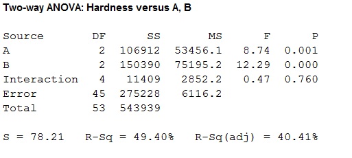
For Factor A, the F-test statistic is 8.74 and the P-value is 0.001.
For Factor B, the F-test statistic is 12.29and the P-value is 0.000.
For interaction, the F-test statistic is 0.47 and the P-value is 0.760.
c.
Explain whether the additive model is plausible.
Answer to Problem 14E
The additive model is plausible.
Explanation of Solution
Calculation:
Interaction:
Null hypothesis:
Alternative hypothesis:
For interaction, the F-test statistic is 0.47 and the P-value is 0.760.
Decision:
If
If
Conclusion:
Interaction:
Here, the P-value is greater than the level of significance.
That is,
Therefore, the null hypothesis is not rejected.
Thus, the interaction is not significant at
Therefore all the interactions are equal to zero.
Thus, the additive model is plausible.
d.
Check whether the effects of travel speed on the hardness can be described by the main effects of travel speed. If so, interpret the main effects by multiple comparisons at the 5% level. If not explain the reason.
Answer to Problem 14E
Yes, the effects of travel speed on the hardness can be described by the main effects of travel speed.
There is sufficient evidence to conclude that the effect of a travel speed of 10 differs from those of both 20 and 30 at
Explanation of Solution
Calculation:
Factor A is travel speed.
Main effect of factor A:
Null hypothesis:
Alternative hypothesis:
For Factor A, the F-test statistic is 8.74 and P- value is 0.001.
Decision:
If
If
Conclusion:
Factor A:
Here, the P-value is less than the level of significance.
That is,
Therefore, the null hypothesis is rejected.
Thus, some of the main effects of factor A are non-zero.
Hence, it is not plausible that the main effects of travel speed on the hardness are equal to zero at
Since, the main effects of travel speed on the hardness are not all equal to zero, the effects of travel speed on the hardness can be described by the main effects of travel speed.
Thus, the effects of travel speed on the hardness can be described by the main effects of travel speed.
The main effects can be interpret using Tukey’s method.
State the hypotheses:
Null hypothesis:
Alternative hypothesis:
Decision:
By Tukey’s method for multiple comparisons,
If
If
Here
From Appendix A table A.9, the upper 5% point of the
For comparing travel speed in 10 mm/s and 20 mm/s:
The 5% critical value is,
Substitute
From part (a), the row effects are
Which is greater than 63.41.
Thus, reject the null hypothesis
Hence, for travel speed in 10 mm/s and 20 mm/s there is travel speed affect the hardness.
For comparing travel speed in 10 mm/s and 30 mm/s:
Which is greater than 63.41.
Thus, reject the null hypothesis
Hence, for travel speed in 10 mm/s and 30 mm/s there is travel speed affect the hardness.
For comparing travel speed in 20 mm/s and 30 mm/s:
Which is less than 63.41.
Thus, fail to reject the null hypothesis
Hence, for travel speed in 20 mm/s and 30 mm/s there is no travel speed affect the hardness.
Conclusion:
There is sufficient evidence to conclude that the effect of a travel speed of 10 differs from those of both 20 and 30 at
e.
Check whether the effects of accelerating voltage on the hardness can be described by the main effects of accelerating voltage. If so, interpret the main effects by multiple comparisons at the 5% level. If not explain the reason.
Answer to Problem 14E
Yes, the effects of accelerating voltage on the hardness can be described by the main effects of accelerating voltage.
There is sufficient evidence to conclude that the effect of an accelerating voltage in 10 volts differs from those of both 25 volts and 50 volts at
Explanation of Solution
Calculation:
Factor B is accelerating voltage.
Main effect of factor B:
Null hypothesis:
Alternative hypothesis:
For Factor B, the F-test statistic is 12.29 and the P-value is 0.000.
Decision:
If
If
Conclusion:
Factor B:
Here, the P-value is less than the level of significance.
That is,
Therefore, the null hypothesis is rejected.
Thus, some of the main effects of factor B are zero.
Hence, it is not plausible that the main effect of accelerating voltage on the hardness are equal to zero at
Since, the main effects of accelerating voltage on the hardness are not equal to zero, the effects of accelerating voltage on the hardness can be described by the main effects of accelerating voltage.
Thus, the effects of accelerating voltage on the hardness can be described by the main effects of accelerating voltage.
The main effects can be interpret using Tukey’s method.
State the hypotheses:
Null hypothesis:
Alternative hypothesis:
Decision:
By Tukey’s method for multiple comparisons,
If
If
Here
From Appendix A table A.9, the upper 5% point of the
For comparing accelerating in 10 volts and 25 volts:
The 5% critical value is,
Substitute
From part (a), the row effects are
Which is greater than 63.41.
Thus, reject the null hypothesis
Hence, for accelerating in 10 volts and 25 volts there is accelerating voltage affect the hardness.
For comparing accelerating in 10 volts and 50 volts:
Which is greater than 63.41.
Thus, reject the null hypothesis
Hence, for accelerating in 10 volts and 50 volts there is accelerating voltage affect the hardness.
For comparing accelerating in 25 volts and 50 volts:
Which is less than 63.41.
Thus, fail to reject the null hypothesis
Hence, for accelerating in 25 volts and 50 volts there is no accelerating voltage affect the hardness.
Conclusion:
There is sufficient evidence to conclude that the effect of an accelerating voltage in 10 volts differs from those of both 25 volts and 50 volts at
Want to see more full solutions like this?
Chapter 9 Solutions
Statistics for Engineers and Scientists - With Access
Additional Math Textbook Solutions
Elementary Statistics: Picturing the World (6th Edition)
Basic Business Statistics, Student Value Edition (13th Edition)
Introduction to Statistical Quality Control
Elementary Statistics: A Step By Step Approach
Elementary Statistics Using Excel (6th Edition)
Basic Business Statistics, Student Value Edition


- Years of Work Experience and number of Job Offers of 10 job-seekers were as follows: Work Exp. 4 2 5 3 7 12 2 5 4 9 No. of Offers 7 1 8 4 13 19 3 11 9 15 a. Fit the regression equation of No. of Job Offers on Years of Work Experience. b. What will be the predicted number of offers for an applicant with 6 years of experience? c. Verify the relationship between the number of job offers and years of work experience using at least two relevant methodsarrow_forwardThe calories and sugar content per serving size of ten brands of breakfast cereal are fitted with a least squares regression line with computer outputs:arrow_forwardconsider the coefficient estimates of the following market model linear regression of general motors (gm) on the S&P500 market returns coefficient estimate std error tvalue pr(>ItI) intercept 0.005860 0.0003704 1.582 0.12412 sp500 0.0904753 0.266702 3.392 0.00196 The number of observations is 32.At the 1% significance level, what is the (1)test statistic value,(2) the critical values (3) decision regarding the null hypothesis that the beta coefficient on the market returns is equal to 1.61arrow_forward
- The Update to the Task Force Report on Blood Pressure Control in Children [12] reported the observed 90th per-centile of SBP in single years of age from age 1 to 17 based on prior studies. The data for boys of average height are given in Table 11.18. Suppose we seek a more efficient way to display the data and choose linear regression to accomplish this task. age sbp 1 99 2 102 3 105 4 107 5 108 6 110 7 111 8 112 9 114 10 115 11 117 12 120 13 122 14 125 15 127 16 130 17 132 Do you think the linear regression provides a good fit to the data? Why or why not? Use residual analysis to justify your answer. Am I supposed to run a residual plot and QQ-plot for this question?arrow_forwardA Ross MAP team is currently developing a regression model to explain the travel expense of HR consulting firms in a month (measured in thousands of dollars). So far, the team has identified the number of consultants, the number of clients, the number of air-travel trips, and the number of trips to high-expense cities (e.g., NYC, Boston, San Jose) as potential independent variables. A partial output of the corresponding regression model is in Figure 1. Use the figure to answer question 4to6 4. What is the R2 and adjusted R2 of the model? 5. What is the standard error of the estimates (serror) in thousands of dollars? 6. Based on what you can learn from this table, what is your assessment about the model? For your information, the firm with the lowest travel expense was $47K and the firm with the highest expense was $125K in the sample data.arrow_forwardThe average asking rent for 10 markets, and the corresponding monthly mortgage on the median priced home (including taxes and insurance) for 10 cities are given in Rent ($) Mortgage ($) City 1 840 539 City 2 1062 1002 City 3 823 626 City 4 779 711 City 5 796 655 City 6 1071 977 City 7 953 776 City 8 851 695 City 9 762 651 City 10 723 654 What is the quadratic regression model to predict the monthly mortgage on the median priced home, using average asking rent? Fill in the coefficient for the Quadratic independent variable (keep 3 decimal points).arrow_forward
- An urban community wants to show that the incidence of breast cancer is higher in their locality than in a neighboring rural area. (PCB levels were found to be higher in the soil of the urban community). If you find that in the urban community 20 out of 200 adult women have breast cancer and that in the rural community 10 out of 150 adult women have it, could you conclude, at a significance level of 0.05, that breast cancer is more prevalent in the urban community?1. The parameter of interest is:2. The hypotheses for this test are:3. The calculated test statistic is:4. The critical region is:5. Draw the critical region (make decision):6. It can be concluded that:arrow_forwardThe y-interept bo of a least-squares regression line has a useful interpretation only if the x-values are either all positive or all negative. Determine if the statement is true or false. Why? If the statement is false, rewrite as a true statement.arrow_forwardSuppose a researcher is interested inthe effectiveness in a new childhood exercise program implemented in a SRS of schools across a particular county. In order to test the hypothesis that the new program decreases BMI (Kg/m2), the researcher takes a SRS of children from schools where the program is employed and a SRS from schools that do not employ the program and compares the results. Assume the following table represents the SRSs of students and their BMIs. Student intervention group BMI (kg/m2) Student control group BMI (kg/m2) A 18.6 A 21.6 B 18.2 B 18.9 C 19.5 C 19.4 D 18.9 D 22.6 E 24.1 F 23.6 A) Assuming that all the necessary conditions are met (normality, independence, etc.) carry out the appropriate statistical test to determine if the new exercise program is effective. Use an alpha level of 0.05. Do not assume equal variances.B) Construct a 95% confidence interval about your estimate for the average difference in BMI between the groups.arrow_forward
- The following data is about the number of turns required to break a certain type of forged alloy bar, as well as the percentages of two alloying elements present in the metal. A) Fit a least squares regression plane and use its equation to estimate the number of turns required to break one of the bars, when x1 = 2.5 and x2 = 12 In the tabley = number of turnsx1 =% of element Ax2 =% of element Barrow_forwardA recent study examined the effects of carbon monoxide exposure on a group of construction workers. The following table presents the numbers of workers who reported various symptoms, along with the shift (morning, evening, or night) that they worked. Morning Shift Evening Shift Night Shift Influenza 19 12 17 Headache 15 33 6 Weakness 12 14 7 Shortness of Breath 6 10 7 Send data to Excel Test the hypothesis of independence. Use the =α0.10 level of significance and the P-value method with the TI-84 Plus calculator. What do you conclude? H0: The shift and reported symptoms are/are not independent. H1: The shift and reported symptoms are/are not independent. This hypothesis test is a left tailed/right tailed/two tailed test.arrow_forwardThe article “Models for Assessing Hoisting Times of Tower Cranes” (A. Leung and C. Tam, Journal of Construction Engineering and Management, 1999: 385–391) presents a model constructed by a stepwise regression procedure to predict the time needed for a tower crane hoisting operation. Twenty variables were considered, and the stepwise procedure chose a nine-variable model. The adjusted R2 for the selected model was 0.73. True or false: a) The value 0.73 is a reliable measure of the goodness of fit of the selected model. b) The value 0.73 may exaggerate the goodness of fit of the model. c) A stepwise regression procedure selects only variables that are of some use in predicting the value of the dependent variable. d) It is possible for a variable that is of no use in predicting the value of a dependent variable to be part of a model selected by a stepwise regression procedure.arrow_forward
 MATLAB: An Introduction with ApplicationsStatisticsISBN:9781119256830Author:Amos GilatPublisher:John Wiley & Sons Inc
 Probability and Statistics for Engineering and th...StatisticsISBN:9781305251809Author:Jay L. DevorePublisher:Cengage Learning
 Statistics for The Behavioral Sciences (MindTap C...StatisticsISBN:9781305504912Author:Frederick J Gravetter, Larry B. WallnauPublisher:Cengage Learning
 Elementary Statistics: Picturing the World (7th E...StatisticsISBN:9780134683416Author:Ron Larson, Betsy FarberPublisher:PEARSON
 The Basic Practice of StatisticsStatisticsISBN:9781319042578Author:David S. Moore, William I. Notz, Michael A. FlignerPublisher:W. H. Freeman
 Introduction to the Practice of StatisticsStatisticsISBN:9781319013387Author:David S. Moore, George P. McCabe, Bruce A. CraigPublisher:W. H. Freeman