
Videos
The article “Sprinkler Technologies, Soil Infiltration, and Runoff” (D. DeBoer and S. Chu, Journal of Irrigation and Drainage Engineering. 2001:234–239) presents a study of the runoff depth (in mm) for various sprinkler types. Each of four sprinklers was tested on each of four days, with two replications per day (there were three replications on a few of the days: these are omitted). It is of interest to determine whether runoff depth varies with sprinkler type: variation from one day to another is not of interest. The data are presented in the following table.
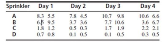
- a. Identify the blocking factor and the treatment factor.
- b. Construct an ANOVA table. You may give
ranges for the P-values. - c. Are the assumptions of a randomized complete block design met? Explain.
- d. Can you conclude that there are differences in
mean runoff depth between some pairs of sprinklers? Explain. - e. Which pairs of sprinklers, if any, can you conclude, at the level, to have differing mean runoff depths?
Want to see the full answer?
Check out a sample textbook solution
Chapter 9 Solutions
STATISTICS FOR ENGR.+SCI-W/ACCESS
Additional Math Textbook Solutions
Intro Stats, Books a la Carte Edition (5th Edition)
Elementary Statistics (13th Edition)
Fundamentals of Statistics (5th Edition)
Statistical Techniques in Business and Economics
Elementary Statistics: Picturing the World (7th Edition)
Statistics: Informed Decisions Using Data (5th Edition)


- An article in the Journal of the Electrochemical Society (Vol. 139, No. 2, 1992, pp. 524–532) describes anexperiment to investigate the low-pressure vapor deposition of polysilicon. The experiment was carried outin a large-capacity reactor at Sematech in Austin, Texas. The reactor has several wafer positions, and fourof these positions are selected at random. The response variable is film thickness uniformity. Threereplicates of the experiment were run, and the data are as follows:a. Test the significance of these wafer position with α=0.05.b. If proven significant, perform a multiple comparison method using Fisher’s LSD.arrow_forwardSuppose a researcher is interested inthe effectiveness in a new childhood exercise program implemented in a SRS of schools across a particular county. In order to test the hypothesis that the new program decreases BMI (Kg/m2), the researcher takes a SRS of children from schools where the program is employed and a SRS from schools that do not employ the program and compares the results. Assume the following table represents the SRSs of students and their BMIs. Student intervention group BMI (kg/m2) Student control group BMI (kg/m2) A 18.6 A 21.6 B 18.2 B 18.9 C 19.5 C 19.4 D 18.9 D 22.6 E 24.1 F 23.6 A) Assuming that all the necessary conditions are met (normality, independence, etc.) carry out the appropriate statistical test to determine if the new exercise program is effective. Use an alpha level of 0.05. Do not assume equal variances.B) Construct a 95% confidence interval about your estimate for the average difference in BMI between the groups.arrow_forwardThe article “Differences in Susceptibilities of Different Cell Lines to Bilirubin Damage” (K. Ngai, C. Yeung, and C. Leung, Journal of Paediatric Child Health, 2000:36–45) reports an investigation into the toxicity of bilirubin on several cell lines. Ten sets of human liver cells and 10 sets of mouse fibroblast cells were placed into solutions of bilirubin in albumin with a 1.4 bilirubin/albumin molar ratio for 24 hours. In the 10 sets of human liver cells, the average percentage of cells surviving was 53.9 with a standard deviation of 10.7. In the 10 sets of mouse fibroblast cells, the average percentage of cells surviving was 73.1 with a standard deviation of 9.1. Find a 98% confidence interval for the difference in survival percentages between the two cell lines.arrow_forward
- classify as either observational or experimental design Heart Failure. In the paper “Cardiac-Resynchronization Therapy with or without an Implantable Defibrillator in Advanced Chronic Heart Failure” (New England Journal of Medicine, Vol. 350, pp. 2140–2150), M. Bristow et al. reported the results of a study of methods for treating patients who had advanced heart failure due to ischemic or nonischemic cardiomyopathies. A total of 1520 patientswere randomly assigned in a 1:2:2 ratio to receive optimal pharmacologic therapy alone or in combination with either a pacemaker or a pacemaker–defibrillator combination. The patients were thenobserved until they died or were hospitalized for any cause.arrow_forwardA study was performed on 200 elementary school students to investigate whether regular Vitamin A supplementation was effective in preventing colds during the month of March. 100 were randomized to receive daily Vitamin A supplements during the month of March, and 100 students were randomized to a placebo group (and did not receive Vitamin A) during the same month. The number of students getting at least one cold in March was computed in the two groups, and the results are given in the following 2 X 2 table. Using a 5% level of significance determine whether there is an association between Vitamin A supplementation and prevention of Common Cold ColdNo Cold Vitamin A1585100 Placebo2575100 40160200arrow_forward3.36 An article in the Journal of the Electrochemical Society (Vol. 139, No. 2, 1992, pp. 524–532) describes an experiment to investigate the low-pressure vapor deposition of polysilicon. The experiment was carried out in a large-capacity reactor at Sematech in Austin, Texas. The reactor has several wafer positions, and four of these positions are selected at random. The response variable is film thickness uniformity. Three replicates of the experiment were run, and the data are as follows: Wafer Position Uniformity 1 2.76 5.67 4.49 2 1.43 1.70 2.19 3 2.34 1.97 1.47 4 0.94 1.36 1.65 (a) Is there a difference in the wafer positions? Use ???? = 0.05. (b) Estimate the variability due to wafer positions. (c) Estimate the random error component. (d) Analyze the residuals from this experiment and comment on model adequacy.arrow_forward
- A U.S. Food Survey showed that Americans routinely eat beef in their diet. Suppose that in a study of 49 consumers in Illinois and 64 consumers in Texas the following results were obtained from two samples regarding average yearly beef consumption: Illinois Texas = 49 = 64 = 54.1lb = 60.4lb S1 = 7.0 S2 = 8.0 Formulate a hypothesis so that, if the null hypothesis is rejected, we can conclude that the average amount of beef eaten annually by consumers in Illinois is significantly less than that eaten by consumers in Texas.arrow_forwardFollowing are the protein contents measured in two types of species:Species 1: 0.72 1.12 0.81 0.89 0.72 0.81 1.01 0.75 0.83Species 2: 1.21 0.93 0.80 1.12 1.22 0.94 0.87 i) Assuming normality, test the hypothesis that the two species have the sameaverage protein contents by using 5-step hypothesis testing procedure at 5 %level of significance, and using the critical values approach.ii) Calculate the p-value of this test and make decision.iii) Write down the standard error of this test and calculate its numerical value ?arrow_forwardConsider the following measurements of blood hemoglobin concentrations (in g/dL) from three human populations at different geographic locations: population1 = [ 14.7 , 15.22, 15.28, 16.58, 15.10 ] population2 = [ 15.66, 15.91, 14.41, 14.73, 15.09] population3 = [ 17.12, 16.42, 16.43, 17.33] What is the standard error of the difference between the means of population 2 and population 3, needed to calculate the Tukey-Kramer q-statistic? What is the Tukey-Kramer q-statistic for populations 2 and 3? (Report the absolute value, if you get a negative number, multiply by -1)arrow_forward
- A paper investigated the driving behavior of teenagers by observing their vehicles as they left a high school parking lot and then again at a site approximately 1 2 mile from the school. Assume that it is reasonable to regard the teen drivers in this study as representative of the population of teen drivers. MaleDriver FemaleDriver 1.4 -0.2 1.2 0.5 0.9 1.1 2.1 0.7 0.7 1.1 1.3 1.2 3 0.1 1.3 0.9 0.6 0.5 2.1 0.5 (a) Use a .01 level of significance for any hypothesis tests. Data consistent with summary quantities appearing in the paper are given in the table. The measurements represent the difference between the observed vehicle speed and the posted speed limit (in miles per hour) for a sample of male teenage drivers and a sample of female teenage drivers. (Use ?males − ?females. Round your test statistic to two decimal places. Round your degrees of freedom down to the nearest whole number. Round your p-value to three decimal places.) t = df =…arrow_forwardA paper investigated the driving behavior of teenagers by observing their vehicles as they left a high school parking lot and then again at a site approximately 1 2 mile from the school. Assume that it is reasonable to regard the teen drivers in this study as representative of the population of teen drivers. MaleDriver FemaleDriver 1.3 -0.3 1.3 0.6 0.9 1.1 2.1 0.7 0.7 1.1 1.3 1.2 3 0.1 1.3 0.9 0.6 0.5 2.1 0.5 (a) Use a .01 level of significance for any hypothesis tests. Data consistent with summary quantities appearing in the paper are given in the table. The measurements represent the difference between the observed vehicle speed and the posted speed limit (in miles per hour) for a sample of male teenage drivers and a sample of female teenage drivers. (Use ?males − ?females. Round your test statistic to two decimal places. Round your degrees of freedom down to the nearest whole number. Round your p-value to three decimal places.) t = df =…arrow_forwardThe authors of the article “Predictive Model for PittingCorrosion in Buried Oil and Gas Pipelines”(Corrosion, 2009: 332–342) provided the data on whichtheir investigation was based.a. Consider the following sample of 61 observations onmaximum pitting depth (mm) of pipeline specimensburied in clay loam soil. 0.41 0.41 0.41 0.41 0.43 0.43 0.43 0.48 0.480.58 0.79 0.79 0.81 0.81 0.81 0.91 0.94 0.941.02 1.04 1.04 1.17 1.17 1.17 1.17 1.17 1.171.17 1.19 1.19 1.27 1.40 1.40 1.59 1.59 1.601.68 1.91 1.96 1.96 1.96 2.10 2.21 2.31 2.462.49 2.57 2.74 3.10 3.18 3.30 3.58 3.58 4.154.75 5.33 7.65 7.70 8.13 10.41 13.44Construct a stem-and-leaf display in which the twolargest values are shown in a last row labeled HI.b. Refer back to (a), and create a histogram based oneight classes with 0 as the lower limit of the firstclass and class widths of .5, .5, .5, .5, 1, 2, 5, and 5,respectively.c. The accompanying comparative boxplot fromMinitab shows plots of pitting depth for four differenttypes of soils.…arrow_forward
 MATLAB: An Introduction with ApplicationsStatisticsISBN:9781119256830Author:Amos GilatPublisher:John Wiley & Sons Inc
 Probability and Statistics for Engineering and th...StatisticsISBN:9781305251809Author:Jay L. DevorePublisher:Cengage Learning
 Statistics for The Behavioral Sciences (MindTap C...StatisticsISBN:9781305504912Author:Frederick J Gravetter, Larry B. WallnauPublisher:Cengage Learning
 Elementary Statistics: Picturing the World (7th E...StatisticsISBN:9780134683416Author:Ron Larson, Betsy FarberPublisher:PEARSON
 The Basic Practice of StatisticsStatisticsISBN:9781319042578Author:David S. Moore, William I. Notz, Michael A. FlignerPublisher:W. H. Freeman
 Introduction to the Practice of StatisticsStatisticsISBN:9781319013387Author:David S. Moore, George P. McCabe, Bruce A. CraigPublisher:W. H. Freeman