
MATLAB: An Introduction with Applications
6th Edition
ISBN: 9781119256830
Author: Amos Gilat
Publisher: John Wiley & Sons Inc
expand_more
expand_more
format_list_bulleted
Related questions
Question
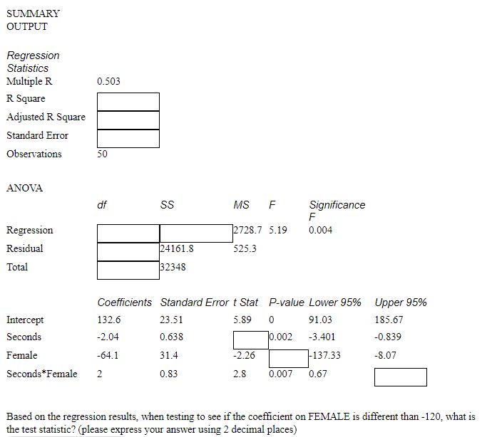

Transcribed Image Text:SUMMARY
OUTPUT
Regression
Statistics
Multiple R
0.503
R Square
Adjusted R Square
Standard Error
Observations
50
ANOVA
df
MS
Significance
F
Regression
2728.7 5.19
0.004
Residual
24161.8
525.3
Total
32348
Coefficients Standard Error t Stat P-value Lower 95% Upper 95%
Intercept
132.6
23.51
5.89 0
91.03
185.67
Seconds
-2.04
0.638
0.002
-3.401
-0.839
Female
-64.1
31.4
-2.26
-137.33
-8.07
Seconds*Female
0.83
2.8
0.007
0.67
Based on the regression results, when testing to see if the coefficient on FEMALE is different than -120, what is
the test statistic? (please express your answer using 2 decimal places)
Expert Solution
This question has been solved!
Explore an expertly crafted, step-by-step solution for a thorough understanding of key concepts.

This is a popular solution

Trending nowThis is a popular solution!

Step by stepSolved in 2 steps

Knowledge Booster

Similar questions
- Table 4.1 SUMMARY OUTPUT Regression Statistics Multiple R R Square Adjusted R Square 0.99794806 Missing 0.99513164 Standard Error 1.64839211 Observations 20 ANOVA Significance F 2.66E-19 af MS F Regression 10561.07486 Missing 16 43.47514498 19 1295.585 Missing 2.717197 Residual Total 10604.55 Coeficients Standard Error t Stat P-Value Intercept 0.562 1.327 0.424 0.677 X1 0.959 0.038 25.245 0.000 X2 1.117 0.125 8.916 0.000 X3 1.460 0.066 22.185 0.000 Consider the output shown in Table 4.1. What is the value of the regression df? 1 3.arrow_forwardConsider the following computer output of a multiple regression analysis relating annual salary to years of education and years of work experience. Regression Statistics Multiple R 0.73360.7336 R Square 0.53810.5381 Adjusted R Square 0.51800.5180 Standard Error 2140.27632140.2763 Observations 49 ANOVA dfdf SSSS MSMS F� Significance F� Regression 22 245,430,999.7671245,430,999.7671 122,715,499.8836122,715,499.8836 26.789226.7892 1.9E-081.9E-08 Residual 4646 210,716,007.0084210,716,007.0084 4,580,782.76114,580,782.7611 Total 4848 456,147,006.7755456,147,006.7755 Coefficients Standard Error t� Stat P-value Lower 95%95% Upper 95%95% Intercept 14276.146814276.1468 2,531.84252,531.8425 5.63865.6386 0.0000010040.000001004 9179.81229179.8122 19,372.481419,372.4814 Education (Years) 2349.95952349.9595 338.5500338.5500 6.94126.9412 0.0000000110.000000011 1668.49371668.4937 3031.42533031.4253 Experience (Years) 833.6183833.6183…arrow_forward|After running the regression analysis between independent and dependent variable the below output is available. SUMMARY OUTPUT Regression Statistics Multiple R 0.714528 R Square 0.510551 Adjusted R Square 0.44937 Standard Error 49.60803 Observations 10 ANOVA ignificance F 1 20536.44 20536.44 8.344902 0.020238 df SS MS F Regression Residual 8 19687.66 2460.957 Total 40224.1 Coefficientsandard Err t Stat P-value Lower 95%Upper 95%ower 95.0%pper 95.0% Intercept -112.208 186.0395 -0.60314 0.563118 -541.216 316.7995 -541.216 316.7995 X Variable 0.398147 0.137827 2.888754 0.020238 0.080319 0.715976 0.080319 0.715976 a. What is the equation of the line? What can you say about the relationship between the two variables?arrow_forward
- Table 4.1 SUMMARY OUTPUT Regression Statistics Multiple R R Square Adjusted R Square 0.99794806 Missing 0.99513164 Standard Error 1.64839211 Observations 20 ANOVA Significance F MS F Regression Missing 10561.07486 16 43.47514498 19 10604.55 fissing 2.717197 1295.585 2.66E-19 Residual Total t Stat Coefficients 0.562 Standard Error P-Value Intercept X1 1.327 0.424 0.677 0.959 0.038 25.245 0.000 X2 1.117 0.125 8.916 0.000 X3 1.460 0.066 22185 0.000 Consider the output shown in Table 4.1. The Mean Square value is missing. What is its actual value? 3520 660 10561 31683arrow_forwardA regression analysis was performed and the summary output is shown below. Regression Statistics Multiple R 0.7802268560.780226856 R Square 0.6087539470.608753947 Adjusted R Square 0.5870180550.587018055 Standard Error 6.7217061336.721706133 Observations 2020 ANOVA dfdf SSSS MSMS F� Significance F� Regression 11 1265.3871265.387 1265.3871265.387 28.006928.0069 4.9549E-054.9549E-05 Residual 1818 813.264813.264 45.18145.181 Total 1919 2078.6512078.651 Step 1 of 2: How many independent variables are included in the regression modelarrow_forwardIf a regression model of the form y= B,+B,x,+... + B,x, is fit to 132 observations on each variable and yields an R´value of 0.87, fill in the blanks in the following ANOVA table. Do all calculations to at least three decimal places. Source of Degrees of freedom Sums of Mean F statistic variation squares squares Regression 69 Error Totalarrow_forward
- Big Time Corporation wanted to determine the relationship between its monthly operating costs and a potential cost driver, machine hours. The output of a regression analysis showed the following information (note: only a portion of the regression analysis results is presented here) SUMMARY OUTPUT Regression Statistics Multiple R 0.998041188 R Square 0.996086212 Adjusted R Square 0.994781616 Standard Error 917.1714273 Observations 5 ANOVA df SS MS F Significance F Regression 1 642276389.7 642276389.7 763.5208906 0.000104039 Residual 3 2523610.281 841203 427 Total 4 644800000 Coefficients Standard Errort Stat P-value Intercept 6679.617454 931.8558049 7.168080532 0.005592948 3714.03639 X Variable 9.796772265 0.354545968 27.63188178 0.000104039 8.66844876 What is variable cost per machine hour (rounded to the nearest cent)? OA. $6,679.62 OB. $917.17 OC. $9.80 OD. $.99 Lower 95% Upper 95.0% 9645.198517 10.92509577arrow_forwardThe parallel trends assumption is a crucial assumption for which the following estimators? Multiple regression Differences-in-Differences First differences Instrumental Variablearrow_forwardUse the final model (attached) to predict the probability of cancer for this patient with the biomarker profile below AFP CEA CA125 CA199 CA50 5.05 10.7 8.12 20.62 57.39arrow_forward
- Are the heights of individuals affected by the heights of their parents. Regression Statistics Multiple R R Square Adjusted R Squar 0.631071992 0.398251859 0.365724932 Standard Error 2.914527039 Observations 40 ANOVA df MS F Significance F Regression Residual 2 208.0084392 104.0042 12.24376 8.30181E-05 37 314.2953108 8.494468 Total 39 522.30375 Coefficients Standard Error t Stat P-value Intercept Mother's Height Father's Height 9.804326378 12.39987353 0.79068 0.43417 0.657952815 0.147476295 4.461414 7.34E-05 0.200358437 0.138223638 1.449524 0.155615 1. Write the regression equation that represents the above equation. 2. Is this a good predictor equation? Why or why not (use appropriate statistics/hypothesis test to prove your point)? 3. Use the equation to predict the height of someone whose mother is 52 inches tall and whose father is 70 inches tall.arrow_forwardItem9 eBook Item 9 The following regression output was obtained from a study of architectural firms. The dependent variable is the total amount of fees in millions of dollars. Predictor Coefficient SE Coefficient t p-value Constant 9.601 3.153 3.045 0.010 x1 0.221 0.110 2.009 0.000 x2 − 1.168 0.577 − 2.024 0.028 x3 − 0.106 0.073 − 1.452 0.114 x4 0.631 0.361 1.748 0.001 x5 − 0.043 0.029 − 1.483 0.112 Analysis of Variance Source DF SS MS F p-value Regression 5 1,844.31 368.9 9.37 0.000 Residual Error 56 2,205.62 39.39 Total 61 4,049.93 x1 is the number of architects employed by the company. x2 is the number of engineers employed by the company. x3 is the number of years involved with health care projects. x4 is the number of states in which the firm operates. x5 is the percent of the firm’s work that is health…arrow_forward
arrow_back_ios
arrow_forward_ios
Recommended textbooks for you
- MATLAB: An Introduction with ApplicationsStatisticsISBN:9781119256830Author:Amos GilatPublisher:John Wiley & Sons Inc
 Probability and Statistics for Engineering and th...StatisticsISBN:9781305251809Author:Jay L. DevorePublisher:Cengage Learning
 Statistics for The Behavioral Sciences (MindTap C...StatisticsISBN:9781305504912Author:Frederick J Gravetter, Larry B. WallnauPublisher:Cengage Learning
  Elementary Statistics: Picturing the World (7th E...StatisticsISBN:9780134683416Author:Ron Larson, Betsy FarberPublisher:PEARSON
 The Basic Practice of StatisticsStatisticsISBN:9781319042578Author:David S. Moore, William I. Notz, Michael A. FlignerPublisher:W. H. Freeman
 Introduction to the Practice of StatisticsStatisticsISBN:9781319013387Author:David S. Moore, George P. McCabe, Bruce A. CraigPublisher:W. H. Freeman
MATLAB: An Introduction with Applications
Statistics
ISBN:9781119256830
Author:Amos Gilat
Publisher:John Wiley & Sons Inc
Probability and Statistics for Engineering and th...
Statistics
ISBN:9781305251809
Author:Jay L. Devore
Publisher:Cengage Learning
Statistics for The Behavioral Sciences (MindTap C...
Statistics
ISBN:9781305504912
Author:Frederick J Gravetter, Larry B. Wallnau
Publisher:Cengage Learning
Elementary Statistics: Picturing the World (7th E...
Statistics
ISBN:9780134683416
Author:Ron Larson, Betsy Farber
Publisher:PEARSON
The Basic Practice of Statistics
Statistics
ISBN:9781319042578
Author:David S. Moore, William I. Notz, Michael A. Fligner
Publisher:W. H. Freeman
Introduction to the Practice of Statistics
Statistics
ISBN:9781319013387
Author:David S. Moore, George P. McCabe, Bruce A. Craig
Publisher:W. H. Freeman