
Concept explainers
Videos
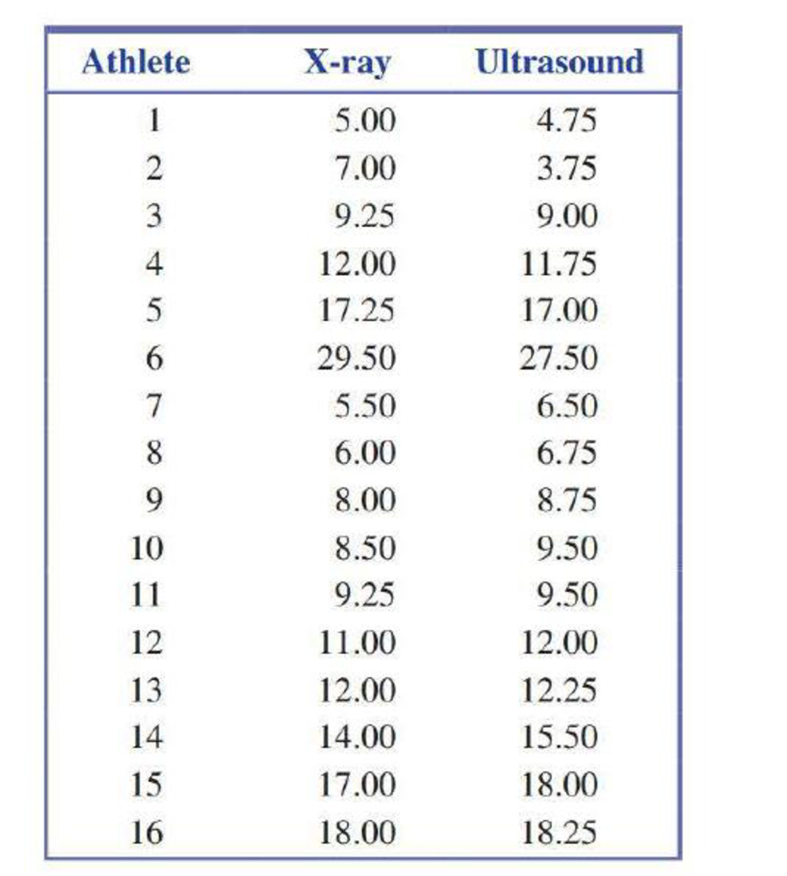
The authors of the paper “Ultrasound Techniques Applied to Body Fat Measurement in Male and Female Athletes” (Journal of Athletic Training [2009]: 142–147) compared two different metods for measuring body fat percentage. One method uses ultrasound, and the other method uses X-ray technology. Body fat percentages using each of these methods for 16 athletes (a subset of the data given in a graph that appeared in the paper) are given in the accompanying table. You can assume that the 16 athletes who participated in this study are representative of the population of athletes. Use these data to estimate the difference in

Trending nowThis is a popular solution!

Chapter 11 Solutions
INTRODUCTION TO STATISTICS & DATA ANALYS


- In a study, 10 healthy men were exposed to diesel exhaust for 1 hour. A measure of brain activity (called median power frequency, or MPF in Hz) was recorded at two different locations in the brain both before and after the diesel exhaust exposure. The resulting data are given in the accompanying table. For purposes of this exercise, assume that the sample of 10 men is representative of healthy adult males. Subject MPF (in Hz) Location 1before Location 1after Location 2before Location 2after 1 6.4 8.0 6.9 9.4 2 8.6 12.7 9.5 11.2 3 7.4 8.4 6.6 10.2 4 8.6 9.0 9.0 9.7 5 9.8 8.4 9.6 9.2 6 8.9 11.0 9.0 11.9 7 9.1 14.4 7.9 9.3 8 7.4 11.1 8.1 9.1 9 6.7 7.3 7.2 8.0 10 8.9 11.2 7.4 9.3 Construct a 90% confidence interval estimate for the difference in mean MPF at brain location 1 (in Hz) before and after exposure to diesel exhaust. (Hint: See Example 13.7.) (Use ?d = ?before − ?after. Use a table or technology. Round your answers to two decimal places.)…arrow_forwardA study was performed on 200 elementary school students to investigate whether regular Vitamin A supplementation was effective in preventing colds during the month of March. 100 were randomized to receive daily Vitamin A supplements during the month of March, and 100 students were randomized to a placebo group (and did not receive Vitamin A) during the same month. The number of students getting at least one cold in March was computed in the two groups, and the results are given in the following 2 X 2 table. Using a 5% level of significance determine whether there is an association between Vitamin A supplementation and prevention of Common Cold ColdNo Cold Vitamin A1585100 Placebo2575100 40160200arrow_forwardIn ongoing economic analyses, the U.S. federal government compares per capita incomes not only among different states but also for the same state at different times. Typically, what the federal government finds is that "poor" states tend to stay poor and "wealthy" states tend to stay wealthy. Would we have been able to predict the 1999 per capita income for a state (denoted by y ) from its 1980 per capita income (denoted by x )? The following bivariate data give the per capita income (in thousands of dollars) for a sample of fourteen states in the years 1980 and 1999 (source: U.S. Bureau of Economic Analysis, Survey of Current Business, May 2000 ). The data are plotted in the scatter plot in Figure 1, and the least-squares regression line is drawn. The equation for this line is =y+0.382.75x . 1980 per capita income, x(in $1000s) 1999 per capita income, y(in $1000s) South Dakota 8.1 25.1 Utah 8.5 23.4 West Virginia 8.2 20.9…arrow_forward
- In ongoing economic analyses, the federal government compares per capita incomes not only among different states but also for the same state at different times. Typically, what the federal government finds is that "poor" states tend to stay poor and "wealthy" states tend to stay wealthy. Would we have gotten information about the 1999 per capita income for a state (denoted by y ) from its 1980 per capita income (denoted by x)? The following bivariate data give the per capita income (in thousands of dollars) for a sample of fifteen states in the years 1980 and 1999 (source: U.S. Bureau of Economic Analysis, Survey of Current Business, May 2000). The data are plotted in the scatter plot in Figure 1. Also given is the product of the 1980 per capita income and the 1999 per capita income for each of the fifteen states. (These products, written in the column labelled " xy ", may aid in calculations.) Question table 1980 per capita income, x (in $1000 s) 1999 per capita…arrow_forwardA paper investigated the driving behavior of teenagers by observing their vehicles as they left a high school parking lot and then again at a site approximately 1 2 mile from the school. Assume that it is reasonable to regard the teen drivers in this study as representative of the population of teen drivers. MaleDriver FemaleDriver 1.3 -0.3 1.3 0.6 0.9 1.1 2.1 0.7 0.7 1.1 1.3 1.2 3 0.1 1.3 0.9 0.6 0.5 2.1 0.5 (a) Use a .01 level of significance for any hypothesis tests. Data consistent with summary quantities appearing in the paper are given in the table. The measurements represent the difference between the observed vehicle speed and the posted speed limit (in miles per hour) for a sample of male teenage drivers and a sample of female teenage drivers. (Use ?males − ?females. Round your test statistic to two decimal places. Round your degrees of freedom down to the nearest whole number. Round your p-value to three decimal places.) t = df =…arrow_forwardBased on a survey of a random sample of 900 adults in the United States, a journalist reports that A random sample of 100 movie goers was asked to state his or her gender and favorite soft drink available at the local movie theater. The results appear in the table below. Is there a relationship between gender and soft drink preference? Coke Diet Coke Sprite Male 23 11 12 Female 16 28 10 To analyze the results, which of the following tests is most appropriate? A)Chi-square test of independence B)Chi-square test of homogeneity C)Two sample t-test D)Matched pair t-test E)Chi-square goodness of fitarrow_forward
- A paper investigated the driving behavior of teenagers by observing their vehicles as they left a high school parking lot and then again at a site approximately 1 2 mile from the school. Assume that it is reasonable to regard the teen drivers in this study as representative of the population of teen drivers. MaleDriver FemaleDriver 1.4 -0.2 1.2 0.5 0.9 1.1 2.1 0.7 0.7 1.1 1.3 1.2 3 0.1 1.3 0.9 0.6 0.5 2.1 0.5 (a) Use a .01 level of significance for any hypothesis tests. Data consistent with summary quantities appearing in the paper are given in the table. The measurements represent the difference between the observed vehicle speed and the posted speed limit (in miles per hour) for a sample of male teenage drivers and a sample of female teenage drivers. (Use ?males − ?females. Round your test statistic to two decimal places. Round your degrees of freedom down to the nearest whole number. Round your p-value to three decimal places.) t = df =…arrow_forwardSuppose a researcher is interested inthe effectiveness in a new childhood exercise program implemented in a SRS of schools across a particular county. In order to test the hypothesis that the new program decreases BMI (Kg/m2), the researcher takes a SRS of children from schools where the program is employed and a SRS from schools that do not employ the program and compares the results. Assume the following table represents the SRSs of students and their BMIs. Student intervention group BMI (kg/m2) Student control group BMI (kg/m2) A 18.6 A 21.6 B 18.2 B 18.9 C 19.5 C 19.4 D 18.9 D 22.6 E 24.1 F 23.6 A) Assuming that all the necessary conditions are met (normality, independence, etc.) carry out the appropriate statistical test to determine if the new exercise program is effective. Use an alpha level of 0.05. Do not assume equal variances.B) Construct a 95% confidence interval about your estimate for the average difference in BMI between the groups.arrow_forwardRecently, researchers have begun to focus on the relationship between potentially toxic environmental exposures in children to a number of adverse health outcomes. Suppose one such researcher wants to investigate the relationship between lead levels in soil (micrograms/dL) and BMI (kg/m2). The following table represents a SRS of households with the corresponding exterior lead levels and BMI of a randomly sampled child in the home. Lead levels BMI 13.6 19.7 14.3 19.9 9.7 20.1 9.4 22.1 11.4 19.8 10.9 21.6 A) Write out the null and alternative hypotheses for a formal test of significance testing the correlation between the two variables and calulate a t statistic and interpret your pvalue and results.arrow_forward
- Low-Birth-Weight Hospital Stays. Data on low-birthweight babies were collected over a 2-year period by 14 participating centers of the National Institute of Child Health and Human Development Neonatal Research Network. Results were reported by J. Lemons et al. in the on-line paper “Very Low Birth Weight Outcomes of the National Institute of ChildHealth and Human Development Neonatal Research Network” (Pediatrics, Vol. 107, No. 1, p. e1). For the 1084 surviving babies whose birth weights were 751– 1000 grams, the average length of stay in the hospital was 86 days, although one center had an average of 66 days and another had an average of 108 days. a. Can the mean lengths of stay be considered population means? Explain your answer.b. Assuming that the population standard deviation is 12 days, determine the z-score for a baby’s length of stay of 86 days at the center where the mean was 66 days.c. Assuming that the population standard deviation is 12 days, determine the z-score for a…arrow_forwardAn automotive engineer is investigating two different types of metering devices for an electronic fuel injection system to determine whether they differ in their fuel mileage performance. The system is installed on 10 different cars, and a test is run with each metering device on each car. The data is provided below: Metering Device Car 1 2 1 17.6 16.8 2 19.4 20.0 3 18.2 17.6 4 17.1 16.4 5 15.3 16.0 6 15.9 15.9 7 16.3 16.5 8 18.0 18.4 9 17.3 16.4 10 19.1 20.1 Is there a significant difference between the means of the two metering devices? Use . Interpret the result in the context of the problem. An article in the journal Hazardous Waste and Hazardous Materials (Vol. 6, 1989) reported the results of an analysis of the weight of calcium in standard cement and cement doped with lead. Reduced levels of calcium would indicate that the hydration mechanism in the cement is blocked…arrow_forwardAn article in the Journal of Quality Technology (Vol. 13, No. 2, 1981, pp. 111–114) describes an experimentthat investigates the effects of four bleaching chemicals on pulp brightness. These four chemicals wereselected at random from a large population of potential bleaching agents. The data are as follows:a. Test the significance of these chemical types with α=0.05.b. If proven significant, perform a multiple comparison method using Fisher’s LSDarrow_forward
 MATLAB: An Introduction with ApplicationsStatisticsISBN:9781119256830Author:Amos GilatPublisher:John Wiley & Sons Inc
 Probability and Statistics for Engineering and th...StatisticsISBN:9781305251809Author:Jay L. DevorePublisher:Cengage Learning
 Statistics for The Behavioral Sciences (MindTap C...StatisticsISBN:9781305504912Author:Frederick J Gravetter, Larry B. WallnauPublisher:Cengage Learning
 Elementary Statistics: Picturing the World (7th E...StatisticsISBN:9780134683416Author:Ron Larson, Betsy FarberPublisher:PEARSON
 The Basic Practice of StatisticsStatisticsISBN:9781319042578Author:David S. Moore, William I. Notz, Michael A. FlignerPublisher:W. H. Freeman
 Introduction to the Practice of StatisticsStatisticsISBN:9781319013387Author:David S. Moore, George P. McCabe, Bruce A. CraigPublisher:W. H. Freeman