Concept explainers
Videos
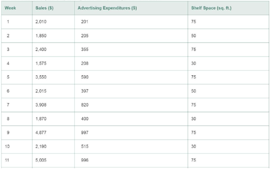
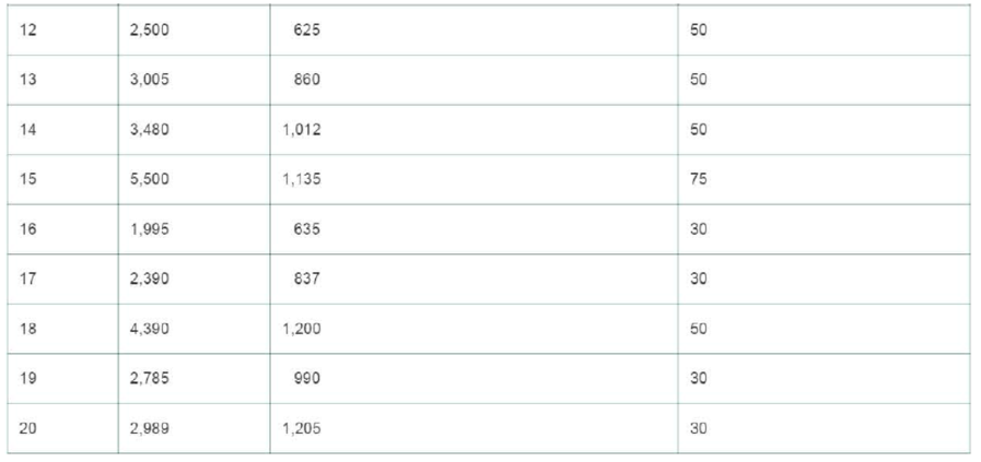
Promotion of supermarket vegetables. A supermarket chain is interested in exploring the relationship between the sales of its store-brand canned vegetables (y), the amount spent on promotion of the vegetables in local newspapers (x1), and the amount of shelf space allocated to the brand (x2). One of the chain's supermarkets was randomly selected, and over a 20-week period x1 and were varied, as reported in the table.
a. Fit the following model to the data:
- b. Conduct an F-test to investigate the overall usefulness of this model. Use a=.05.
- c. Test for the presence of interaction between advertising expenditures and shelf space. Use α= 05.
- d. Explain what it means to say that advertising expenditures and shelf space interact.
- e. Explain how you could be misled by using a first-order model instead of an interaction model to explain how advertising expenditures and shelf space influence sales.
- f. Based on the type of data collected, comment on the assumption of independent errors.

Trending nowThis is a popular solution!

Chapter 12 Solutions
Statistics Plus New MyLab Statistics with Pearson eText -- Access Card Package (13th Edition)


- Urban Travel Times Population of cities and driving times are related, as shown in the accompanying table, which shows the 1960 population N, in thousands, for several cities, together with the average time T, in minutes, sent by residents driving to work. City Population N Driving time T Los Angeles 6489 16.8 Pittsburgh 1804 12.6 Washington 1808 14.3 Hutchinson 38 6.1 Nashville 347 10.8 Tallahassee 48 7.3 An analysis of these data, along with data from 17 other cities in the United States and Canada, led to a power model of average driving time as a function of population. a Construct a power model of driving time in minutes as a function of population measured in thousands b Is average driving time in Pittsburgh more or less than would be expected from its population? c If you wish to move to a smaller city to reduce your average driving time to work by 25, how much smaller should the city be?arrow_forwardOlympic Pole Vault The graph in Figure 7 indicates that in recent years the winning Olympic men’s pole vault height has fallen below the value predicted by the regression line in Example 2. This might have occurred because when the pole vault was a new event there was much room for improvement in vaulters’ performances, whereas now even the best training can produce only incremental advances. Let’s see whether concentrating on more recent results gives a better predictor of future records. (a) Use the data in Table 2 (page 176) to complete the table of winning pole vault heights shown in the margin. (Note that we are using x=0 to correspond to the year 1972, where this restricted data set begins.) (b) Find the regression line for the data in part ‚(a). (c) Plot the data and the regression line on the same axes. Does the regression line seem to provide a good model for the data? (d) What does the regression line predict as the winning pole vault height for the 2012 Olympics? Compare this predicted value to the actual 2012 winning height of 5.97 m, as described on page 177. Has this new regression line provided a better prediction than the line in Example 2?arrow_forward
 Functions and Change: A Modeling Approach to Coll...AlgebraISBN:9781337111348Author:Bruce Crauder, Benny Evans, Alan NoellPublisher:Cengage Learning
 College AlgebraAlgebraISBN:9781305115545Author:James Stewart, Lothar Redlin, Saleem WatsonPublisher:Cengage Learning
 Linear Algebra: A Modern IntroductionAlgebraISBN:9781285463247Author:David PoolePublisher:Cengage Learning
 Glencoe Algebra 1, Student Edition, 9780079039897...AlgebraISBN:9780079039897Author:CarterPublisher:McGraw Hill