Videos
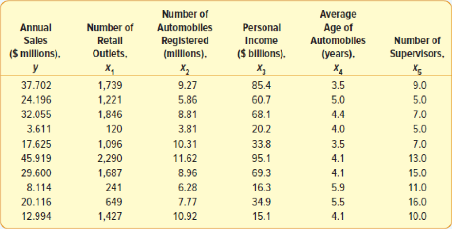
Suppose that the sales manager of a large automotive parts distributor wants to estimate the total annual sales for each of the company’s regions. Five factors appear to be related to regional sales: the number of retail outlets in the region, the number of automobiles in the region registered as of April 1, the total personal income recorded in the first quarter of the year, the average age of the automobiles (years), and the number of sales supervisors in the region. The data for each region were gathered for last year. For example, see the following table. In region 1 there were 1,739 retail outlets stocking the company’s automotive parts, there were 9,270,000 registered automobiles in the region as of April 1, and so on. The region’s sales for that year were $37,702,000.
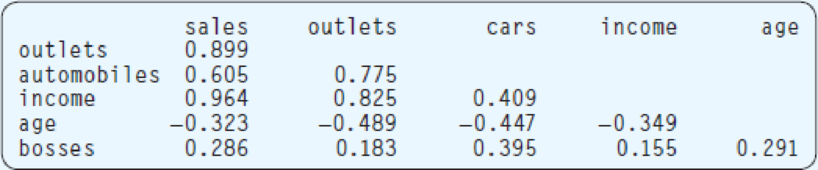
- a. Consider the following correlation matrix. Which single variable has the strongest correlation with the dependent variable? The
correlations between the independent variables outlets and income and between outlets and number of automobiles are fairly strong. Could this be a problem? What is this condition called?
- b. The output for all five variables is shown below. What percent of the variation is explained by the regression equation?
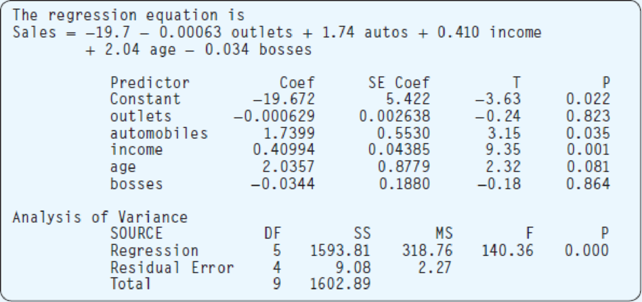
- c. Conduct a global test of hypothesis to determine whether any of the regression coefficients are not zero. Use the .05 significance level.
- d. Conduct a test of hypothesis on each of the independent variables. Would you consider eliminating “outlets” and “bosses”? Use the .05 significance level.
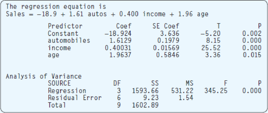
- e. The regression has been rerun below with “outlets” and “bosses” eliminated. Compute the coefficient of determination. How much has R2 changed from the previous analysis?
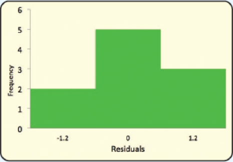
- f. Following is a histogram of the residuals. Does the normality assumption appear reasonable? Why?
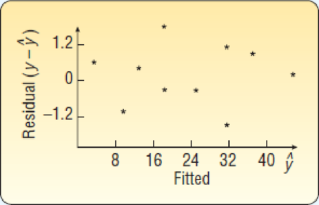
- g. Following is a plot of the fitted values of y (i.e.,
a.
Find the single variable that has the strongest correlation with the dependent variable.
Explain whether the fairly strong correlations between outlets and income and outlets and number of automobiles, will be any problem.
Provide the name of the condition.
Answer to Problem 18CE
The single variable that has the strongest correlation with the dependent variable, is “income”.
The name of the condition is multicollinearity.
Explanation of Solution
Multiple linear regression model:
A multiple linear regression model is given as
Here, a is the intercept term of the regression model, that is, the value of predicted value of y when X’s are 0 and
In the given problem the predicted dependent variable y is the annual sales. The number of retail outlets, the number of automobiles registered, personal income, the average of automobiles and the number of supervisors, are defined as
Correlation:
The correlation between two variables measures the linear relationship between those two variables.
According to the given output there is a strongest correlation between the independent variable “income” and the dependent variable “sales”. The correlation coefficient between “income” and “sales” is 0.964.
Thus, it implies that as the personal income increases the annual sales also increase.
Multicollinearity:
In a multiple regression model, when there is high correlation between two or more independent variables, then multicollinearity occurs.
The correlation between the independent variables outlets and income and between outlets and number of automobiles are fairly strong, such as, 0.825 and 0.775, respectively.
These correlations can occur multicollinearity in the regression model.
Due to this multicollinearity the standard errors will be high and there will be no exact estimate of the partial regression coefficient. Moreover, there will be difficulty to measure the relative significance of independent variables.
b.
Find the percent of the variation that is explained by the regression equation.
Answer to Problem 18CE
The approximate value of coefficient of multiple determination is 99.43%, that is, 99.43% of the variation is explained by the regression equation.
Explanation of Solution
Calculation:
According to an ANOVA table the coefficient of multiple determination is defined as,
Where SSR is the regression sum of squares and SS total is the total sum of square.
According to the output the SSR and SS total are 1,593.91 and 1,602.89, respectively.
Hence, the coefficient of multiple determination is,
Thus, the approximate value of coefficient of multiple determination is 99.43%.
Hence, 99.43% of the variation is explained by the regression equation.
c.
Perform a global hypothesis test to check whether any of the regression coefficients is not zero at 0.05 significance level.
Answer to Problem 18CE
There is strong evidence that at least any of the regression coefficient is not 0 at 0.05 significance level.
Explanation of Solution
Calculation:
Consider that y is dependent variable and
State the hypotheses:
Null hypothesis:
That is, the model is not significant.
Alternative hypothesis:
That is, the model is significant.
In case of global test the F test statistic is defined as,
According to the output, the value of F statistic is 140.36 with numerator degrees of freedom 5 and denominator degrees of freedom 5.
The level of significance is
Decision rule:
- If
- Otherwise failed to reject the null hypothesis.
Conclusion:
Here, p-value corresponding to the global test is 0.
Hence,
That is, the p-value is less than the level of significance.
Therefore, reject the null hypothesis.
Hence, it can be concluded that at least any of the regression coefficient is not 0 at 0.05 significance level.
d.
Perform individual tests of each independent variable at 0.05 significance level.
Explain whether the independent variables “outlets” and “bosses” will be eliminated.
Answer to Problem 18CE
There is no significant relation between y and
The independent random variables “the number of retail outlets”, “average age of automobiles” and “number of supervisors” can be eliminated.
Explanation of Solution
Calculation:
For independent variable
Consider that
State the hypotheses:
Null hypothesis:
That is, there is no significant relationship between y and
Alternative hypothesis:
That is, there is significant relationship between y and
In case of individual regression coefficient test the t test statistic is defined as,
According to the given information the t statistic value corresponding to
The level of significance is
Decision rule:
- If
- Otherwise failed to reject the null hypothesis.
Conclusion:
Here, p-value corresponding to the outlets
Hence,
That is, the p-value is greater than the level of significance.
Therefore, fail to reject the null hypothesis.
Hence, it can be concluded that there is no significant relationship between y and
For independent variable
Consider that
State the hypotheses:
Null hypothesis:
That is, there is no significant relationship between y and
Alternative hypothesis:
That is, there is significant relationship between y and
According to the given ANOVA table the value of t test statistic corresponding to
Conclusion:
Here, p-value corresponding to the automobiles
Hence,
That is, the p-value is less than the level of significance.
Therefore, reject the null hypothesis.
Hence, it can be concluded that there is significant relationship between y and
For independent variable
Consider that
State the hypotheses:
Null hypothesis:
That is, there is no significant relationship between y and
Alternative hypothesis:
That is, there is significant relationship between y and
According to the given ANOVA table the value of t test statistic corresponding to
Conclusion:
Here, p-value corresponding to the income
Hence,
That is, the p-value is less than the level of significance.
Therefore, reject the null hypothesis.
Hence, it can be concluded that there is significant relationship between y and
For independent variable
Consider that
State the hypotheses:
Null hypothesis:
That is, there is no significant relationship between y and
Alternative hypothesis:
That is, there is significant relationship between y and
According to the given ANOVA table the value of t test statistic corresponding to
Conclusion:
Here, p-value corresponding to the age
Hence,
That is, the p-value is greater than the level of significance.
Therefore, fail to reject the null hypothesis.
Hence, it can be concluded that there is no significant relationship between y and
For independent variable
Consider that
State the hypotheses:
Null hypothesis:
That is, there is no significant relationship between y and
Alternative hypothesis:
That is, there is significant relationship between y and
According to the given ANOVA table the value of t test statistic corresponding to
Conclusion:
Here, p-value corresponding to the bosses
Hence,
That is, the p-value is greater than the level of significance.
Therefore, fail to reject the null hypothesis.
Hence, it can be concluded that there is no significant relationship between y and
As there are no significant relationship between the dependent variable and the independent variables
Hence, it can be said that there is no significant relationship between the annual sales and the number of retail outlets and the number of supervisors. Thus, it is better to omit these independent random variables “the number of retail outlets” and “the number of supervisors”.
Moreover, there is no significant relationship between the dependent variable and the independent variable
Hence, it can be said that there is no significant relationship between the annual sales and the average age of automobiles. Thus, it is better to omit this independent random variable “average age of automobiles” also.
e.
Find the coefficient of determination.
Find the change of
Answer to Problem 18CE
The approximate value of coefficient of multiple determination is 99.43%, that is, 99.43% of the variation is explained by the regression equation.
Explanation of Solution
Calculation:
According to an ANOVA table the coefficient of multiple determination is defined as,
Where SSR is the regression sum of squares and SS total is the total sum of square.
According to the output after eliminating “outlets” and “bosses”, the SSR and SS total are 1,593.66 and 1,602.89, respectively.
Hence, the coefficient of multiple determination is,
Thus, the approximate value of coefficient of multiple determination is 99.42%.
Hence, there is only 0.01%
f.
Explain whether the normality assumptions appear reasonably.
Explanation of Solution
Assumption of normality from histogram:
- The majority of the observation in the middle and centered on the mean of 0.
- There are lower frequencies on the tails of the distributions.
According to the given histogram, the most of the observations are centered on the mean of 0 and there are less frequencies on the tails of the distributions.
Hence, the normality assumptions appear reasonably.
g.
Explain about the residual plot and also explain whether any assumptions are violated.
Explanation of Solution
Assumption for residual analysis for the regression model:
- The plot of the residuals vs. the observed values of the predictor variable should fall roughly in a horizontal band and symmetric about x-axis.
- For a normal probability plot, residuals should be roughly linear.
- There should not be any observable pattern.
According to the given residual plot, the points are roughly in a horizontal band and more or less symmetric about x-axis. Moreover, there is no particular pattern in the residual plot. A complete haphazard and random nature has observed.
Hence, the assumptions of the residual plot are not violated.
Want to see more full solutions like this?
Chapter 14 Solutions
EBK STATISTICAL TECHNIQUES IN BUSINESS


- What is the total effect on the economy of a government tax rebate of $500 to each household in order to stimulate the economy if each household will spend of the rebate in goods and services?arrow_forwardTo allocate annual bonuses, a manager must choose his top four employees and rank them first to fourth. In how many ways can he create the ‘Top- Four” list out of the 32 employees?arrow_forward
 Glencoe Algebra 1, Student Edition, 9780079039897...AlgebraISBN:9780079039897Author:CarterPublisher:McGraw Hill