
Videos
a.
Make the correlation matrix.
Find the independent variables those have strong or weak
Explain whether there are any problems with multicollinearity.
Also explain whether it is surprising that the
a.
Answer to Problem 34DA
The correlation matrix is obtained as,
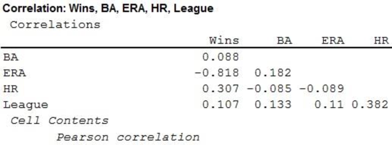
There are no problems of multicollinearity.
Explanation of Solution
Multiple linear regression model:
A multiple linear regression model is given as
Here, a is the intercept term of the regression model, that is, the value of predicted value of y when X’s are 0 and
In the given problem the predicted dependent variable y is the number of won games. The team batting average (BA), the team earned run average (ERA), the number of home runs (HR) and whether the team plays in the American or the National League, are denoted as
Step by step procedure to obtain the correlation matrix using MINITAB software is given below:
- Choose Stat > Basic Statistics > Correlation.
- Select the columns of Wins, BA, ERA, HR and League under Variables tab.
- Click OK.
The MINITAB output is obtained.
According to the obtained output there is a strong correlation between the independent variable “ERA”, and the dependent variable “Wins”. That is, –0.818. Hence, it can be sad that if the team earned run average is decreased due to better pitching then the number of Wins is increased and vice versa. This is not surprising.
Multicollinearity:
In a multiple regression model, when there is high correlation between two or more independent variables, then multicollinearity occurs.
The correlation coefficients between the independent variables are moderate, which does not indicate any presence of multicollinearity.
b.
Find the regression equation and explain the procedure of the selection of the variables to include in the equation.
Explain the correlation analysis.
Prove that the regression equation shows a significant relationship.
Give the regression equation and interpret the practical interpretation of it.
Find and interpret
Explain whether the number of wins affected by whether the team plays in the National or the American League.
b.
Explanation of Solution
Calculation:
Step by step procedure to obtain the regression equation using MINITAB software:
- Choose Stat > Regression > Regression > Fit Regression Model.
- Under Responses, enter the column of Wins.
- Under Continuous predictors, enter the columns of BA, ERA, HR, and League.
- Click OK.
Output using MINITAB software is given below:
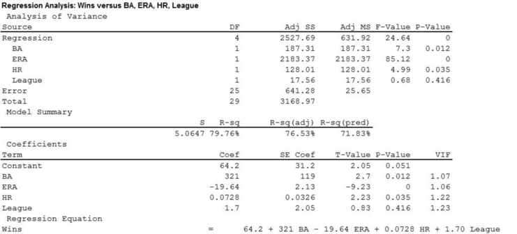
Now, it is known that if the p-value of an independent variable is less than the level of significance then there is significant relation between the dependent variable and that independent variable. Otherwise, there is no significant relationship.
Consider that, the level of significance is
According to the correlation analysis one can omit that independent variable, which has the lowest correlation with the dependent variable.
Hence, in this case one can omit “League” from the
Thus, for revised regression analysis the dependent variable is “Wins” (y) and the independent variables are “BA”
Step by step procedure to obtain the regression equation using MINITAB software:
- Choose Stat > Regression > Regression > Fit Regression Model.
- Under Responses, enter the column of Wins.
- Under Continuous predictors, enter the columns of BA, ERA, and HR.
- Click OK.
- Choose Graphs.
- Under Residual plot select Histogram of residuals and Residual Versus fit.
- Click OK.
- Click OK.
Output using MINITAB software is given below:
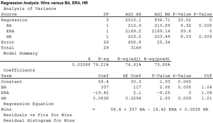
Hence, the revised regression equation is
Hence, it can be said that if batting average is increased by 1 unit then 0.337 matches will be won more. However, if the team home run is increased by 1 unit the inly 0.0838 matches can be won. In addition, for 1 unit decrease in team earned run average the number of match won increased by 19.42.
The coefficient of determination (
c.
Perform a global test on the set of the independent variables and interpret.
c.
Explanation of Solution
Consider that y is dependent variable and
State the hypotheses:
Null hypothesis:
That is, the model is not significant.
Alternative hypothesis:
That is, the model is significant.
In case of global test the F test statistic is defined as,
According to the output in Part (a) the value of F statistic is 33.02 with numerator degrees of freedom 3 and denominator degrees of freedom 26.
Consider, the level of significance is
Decision rule:
- If
- Otherwise failed to reject the null hypothesis.
Conclusion:
Here, p-value corresponding to the global test is 0.
Hence,
That is, the p-value is less than the level of significance.
Therefore, reject the null hypothesis.
Hence, it can be concluded that any of the regression coefficient differ from 0 at 0.05 significance level.
d.
Perform a hypothesis test on individual variables.
Explain whether any of the independent variables will be deleted.
d.
Answer to Problem 34DA
There is no need to delete any independent variables.
Explanation of Solution
For independent variable
Consider that
State the hypotheses:
Null hypothesis:
That is, there is no significant relationship between y and
Alternative hypothesis:
That is, there is significant relationship between y and
In case of individual regression coefficient test the t test statistic is defined as,
According to the output in Part (a) the t statistic value corresponding to
Conclusion:
Here, p-value corresponding to the “BA”
Hence,
That is, the p-value is less than the level of significance.
Therefore, reject the null hypothesis.
Hence, it can be concluded that there is significant relationship between y and
For independent variable
Consider that
State the hypotheses:
Null hypothesis:
That is, there is no significant relationship between y and
Alternative hypothesis:
That is, there is significant relationship between y and
According to the output in Part (a) the value of t test statistic corresponding to
Conclusion:
Here, p-value corresponding to the “ERA”
Hence,
That is, the p-value is less than the level of significance.
Therefore, reject the null hypothesis.
Hence, it can be concluded that there is significant relationship between y and
For independent variable
Consider that
State the hypotheses:
Null hypothesis:
That is, there is no significant relationship between y and
Alternative hypothesis:
That is, there is significant relationship between y and
According to the output in Part (a) the value of t test statistic corresponding to
Conclusion:
Here, p-value corresponding to the “HR”
Hence,
That is, the p-value is less than the level of significance.
Therefore, reject the null hypothesis.
Hence, it can be concluded that there is significant relationship between y and
As there are significant relationship between the dependent variable and all of the independent variables, then there is no need to delete any independent variables.
e.
Draw a histogram or a stem-and-leaf display of the residuals from the final regression equation developed in Part (b).
Explain whether it is reasonable to conclude that the normality assumption has been met.
e.
Explanation of Solution
Histogram:
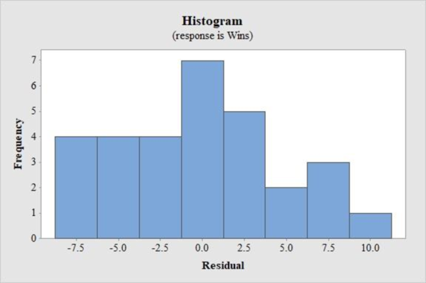
From Part (b), the histogram is obtained as,

Assumption of normality from histogram:
- The majority of the observation in the middle and centered on the mean of 0.
- There are lower frequencies on the tails of the distributions.
According to the given histogram, the most of the observations are centered on the mean of 0 and there are less frequencies on the tails of the distributions. It can be considered as somehow symmetric.
Hence, the normality assumptions appear.
e.
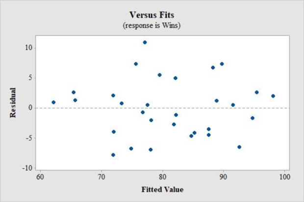
Plot the residuals against the fitted value.
e.
Explanation of Solution
From Part (b), the residual plot is obtained as,

Assumption for residual analysis for the regression model:
- The plot of the residuals vs. the observed values of the predictor variable should fall roughly in a horizontal band and symmetric about x-axis.
- For a normal probability plot, residuals should be roughly linear.
- There should not be any observable pattern.
According to the given residual plot, the points are roughly in a horizontal band and more or less symmetric about x-axis. Moreover, there is no particular pattern in the residual plot. A complete haphazard and random nature has observed. The variability among the residuals is more or less same thorough the whole plot.
Want to see more full solutions like this?
Chapter 14 Solutions
EBK STATISTICAL TECHNIQUES IN BUSINESS


 Glencoe Algebra 1, Student Edition, 9780079039897...AlgebraISBN:9780079039897Author:CarterPublisher:McGraw Hill
 Big Ideas Math A Bridge To Success Algebra 1: Stu...AlgebraISBN:9781680331141Author:HOUGHTON MIFFLIN HARCOURTPublisher:Houghton Mifflin Harcourt