
Concept explainers
Videos
This exercise requires the use of a statistical software package. The authors of the article “Absolute Versus per Unit Body Length Speed of Prey as an Estimator of Vulnerability to Predation” (Animal Behaviour [1999]: 347-352) found that the speed of a prey (twips/s) and the length of a prey (twips × 100) are good predictors of the time (seconds) required to catch the prey. (A twip is a measure of distance used by programmers.) Data were collected in an experiment in which subjects were asked to “catch” an animal of prey moving across his or her computer screen by clicking on it with the mouse. The investigators varied the length of the prey and the speed with which the prey moved across the screen.
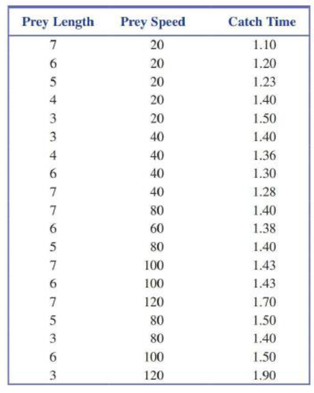
The following data are consistent with summary values and a graph given in the article. Each value represents the average catch time over all subjects. The order of the various speed-length combinations was randomized for each subject.
- a. Fit a multiple regression model for predicting catch time using prey length and speed as predictors.
- b. Predict the catch time for an animal of prey whose length is 6 and whose speed is 50.
- c. Is the multiple regression model useful for predicting catch time? Test the relevant hypotheses using α = 0.05.
- d. The authors of the article suggest that a simple linear regression model with the single predictor
might be a better model for predicting catch time. Calculate these x values and use them to fit a simple linear regression model.
- e. Which of the two models considered (the multiple regression model from Part (a) or the simple linear regression model from Part (d)) would you recommend for predicting catch time? Justify your choice.
a.
Calculate the multiple regression equation.
Answer to Problem 27E
The multiple regression equation is as follows:
Explanation of Solution
Calculation:
The data are about the average catch time over all the subjects.
Software procedure:
Step-by-step procedure to obtain the regression equation using the MINITAB software:
- Choose Stat > Regression > Regression > Fit Regression Model.
- Enter the column of Catch Time under Responses.
- Enter the columns of Prey Length and Prey Speed under Continuous predictors.
- Choose Results and select Analysis of variance, Regression Equation, coefficients, and Model summary.
- Click OK in all dialogue boxes.
Output obtained using the MINITAB software is given below:
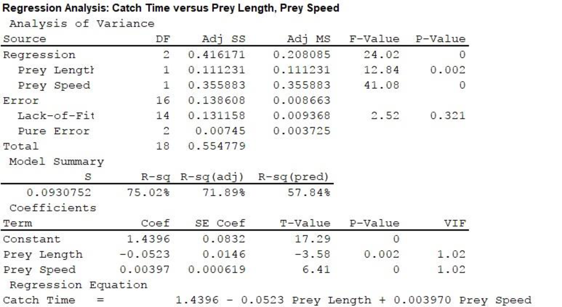
From the MINITAB output, the multiple regression equation is as follows:
b.
Estimate the catch time for an animal.
Answer to Problem 27E
The estimated catch time is 1.3243 seconds.
Explanation of Solution
Calculation:
It is given that the prey length is 6 and the prey speed is 50.
From Part a., the multiple regression equation is as given below:
The estimated catch time for an animal is calculated as follows:
Thus, the estimated catch time is 1.3243 seconds.
c.
Explain whether the multiple regression model is useful to predict the catch time or not at the 0.05 level of significance.
Answer to Problem 27E
There is convincing evidence that at least one of the predictors’ prey length and prey speed are useful for predicting the catch time at the 0.05 level of significance.
Explanation of Solution
Calculation:
1.
The model is
Here, the variable y is the catch time,
2.
Null hypothesis:
That is, there is no useful regression model for predicting catch time.
3.
Alternative hypothesis:
That is, there is useful regression model for predicting the catch time.
4.
Here, the significance level is
5.
Test statistic:
Here, n is the sample size and k is the number of variables in the model.
6.
Assumptions:
Software procedure:
Step-by-step procedure to obtain normal probability plot using the MINITAB software:
- Choose Stat > Regression > Regression > Fit Regression Model.
- Enter the column of Catch Time under Responses.
- Enter the columns of Prey Length and Prey Speed under Continuous predictors.
- Choose Graphs, select Standardized under Residual for plots.
- Choose Normal probability plot of residuals under Residuals plot.
- Click on OK.
- In Graph, click on y-axis. In Type, choose Score under Scale Type.
- Under Scale, Choose Transpose Y and X.
- Click OK.
Output obtained using the MINITAB software is given below:
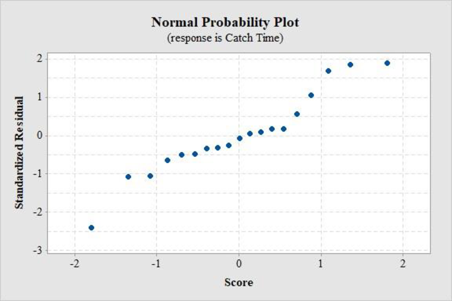
From the MINITAB output, the plot shows a slight linear pattern. Therefore, it can be assumed that the random deviations are distributed normally.
7.
Calculation:
From the MINITAB output in Part a., the F test statistic value for regression is 24.02.
8.
P-value:
From the MINITAB output in Part a., the P-value for regression is 0.
9.
Conclusion:
If
Therefore, the P-value of 0 is less than the 0.05 level of significance.
Hence, reject the null hypothesis.
Thus, there is convincing evidence that at least one of the predictors’ prey length and prey speed are useful for predicting the catch time at the 0.05 level of significance.
d.
Calculate the values of x and fit a simple linear regression model.
Answer to Problem 27E
The values of x are tabulated below:
| Prey Length | Prey Speed | Catch Time | x |
| 7 | 20 | 1.1 | 0.35000 |
| 6 | 20 | 1.2 | 0.30000 |
| 5 | 20 | 1.2 | 0.25000 |
| 4 | 20 | 1.4 | 0.20000 |
| 3 | 20 | 1.5 | 0.15000 |
| 3 | 40 | 1.4 | 0.07500 |
| 4 | 40 | 1.4 | 0.10000 |
| 6 | 40 | 1.3 | 0.15000 |
| 7 | 40 | 1.3 | 0.17500 |
| 7 | 80 | 1.4 | 0.08750 |
| 6 | 60 | 1.4 | 0.10000 |
| 5 | 80 | 1.4 | 0.06250 |
| 7 | 100 | 1.4 | 0.07000 |
| 6 | 100 | 1.4 | 0.06000 |
| 7 | 120 | 1.7 | 0.05833 |
| 5 | 80 | 1.5 | 0.06250 |
| 3 | 80 | 1.4 | 0.03750 |
| 6 | 100 | 1.5 | 0.06000 |
| 3 | 120 | 1.9 | 0.02500 |
The simple linear equation is
Explanation of Solution
Calculation:
It is given that the single predictor x is defined as given below:
The values of x are calculated as follows:
For catch time 1.1:
Substitute the values of prey length as 7 and the prey speed as 20 in x.
Similarly, the remaining values of x are calculated and tabulated as follows:
| Prey Length | Prey Speed | Catch Time | x |
| 7 | 20 | 1.1 | 0.35000 |
| 6 | 20 | 1.2 | 0.30000 |
| 5 | 20 | 1.2 | 0.25000 |
| 4 | 20 | 1.4 | 0.20000 |
| 3 | 20 | 1.5 | 0.15000 |
| 3 | 40 | 1.4 | 0.07500 |
| 4 | 40 | 1.4 | 0.10000 |
| 6 | 40 | 1.3 | 0.15000 |
| 7 | 40 | 1.3 | 0.17500 |
| 7 | 80 | 1.4 | 0.08750 |
| 6 | 60 | 1.4 | 0.10000 |
| 5 | 80 | 1.4 | 0.06250 |
| 7 | 100 | 1.4 | 0.07000 |
| 6 | 100 | 1.4 | 0.06000 |
| 7 | 120 | 1.7 | 0.05833 |
| 5 | 80 | 1.5 | 0.06250 |
| 3 | 80 | 1.4 | 0.03750 |
| 6 | 100 | 1.5 | 0.06000 |
| 3 | 120 | 1.9 | 0.02500 |
Software procedure:
Step-by-step procedure to obtain the regression equation using the MINITAB software:
- Choose Stat > Regression > Regression > Fit Regression Model.
- Enter the column of Catch Time under Responses.
- Enter the columns of x under Continuous predictors.
- Choose Results and select Analysis of variance, Regression Equation, coefficients, and Model summary.
- Click OK in all dialogue boxes.
Output obtained using the MINITAB software is given below:
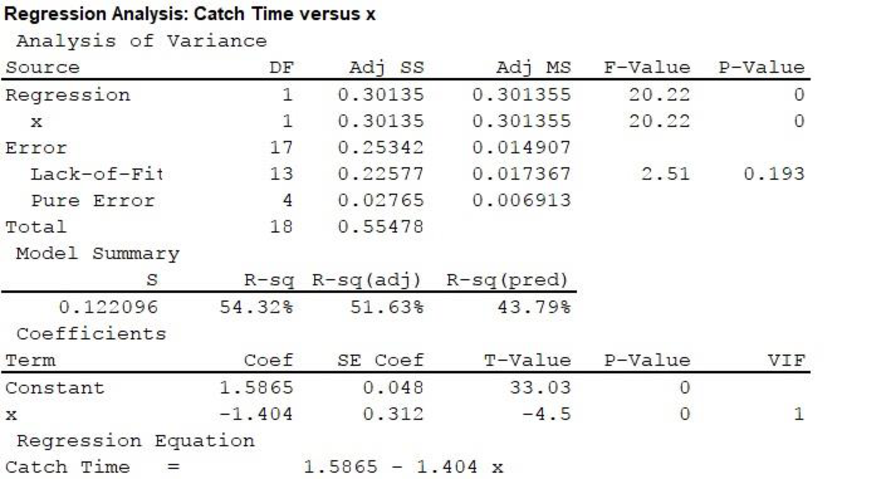
From the MINITAB output, the simple linear regression equation is as follows:
e.
Explain the recommendable regression model.
Explanation of Solution
From Part a., the multiple regression equation is as follows:
From Part d., the simple linear equation is
From the MINITAB output in Part a., the value of
From the MINITAB output in Part d., the value of
By observing these values, the values of
Want to see more full solutions like this?
Chapter 14 Solutions
INTRODUCTION TO STATISTICS & DATA ANALYS


- Consider the following data: Fit a line, y = x1 + x2t, to the data using the least squares approach.arrow_forwardA researcher obtains t(20) = 2.00 and MD = 9 for a repeated-measures study. If the researcher measures effect size using the percentage of variance accounted for, what value will be obtained for r2?arrow_forwardSuppose researchers perform a two-tailed study and the following results are obtained.α=0.05t=2.44df=40Use the t-table to decide if there is a statistically significant difference between the data sets.arrow_forward
- A researcher conducts an independent- measures research study and obtains t = 2.070 with df = 28. How many individuals participated in the entire research study? Using a two- tailed test with α = .05, is there a significant difference between the two treatment conditions? Compute r2 to measure the percentage of variance accounted for by the treatment effect.arrow_forwardA researcher conducts an experiment comparing two methods of teaching young children to read. An older method is compared with a newer one, and the mean performance of the new method was found to be greater than that of the older method The results are reported as follows: t(120) = 2.10, p = .04, (d =.34). a. Are the results statistically significant?arrow_forward
 Glencoe Algebra 1, Student Edition, 9780079039897...AlgebraISBN:9780079039897Author:CarterPublisher:McGraw Hill
 Big Ideas Math A Bridge To Success Algebra 1: Stu...AlgebraISBN:9781680331141Author:HOUGHTON MIFFLIN HARCOURTPublisher:Houghton Mifflin Harcourt