Chapter 2, Problem 153E

(a)

To determine

To find: The marginal total of the provided data to add them in the table.

Answer to Problem 153E

Solution: The obtained marginal totals are shown in the below table.

Field of study	Canada	France	Germany	Italy	Japan	UK	US	Total`
SsBL	64	153	66	125	250	152	878	1688
SME	35	111	66	80	136	128	355	911
AH	27	74	33	42	123	105	397	801
Ed	20	45	18	16	39	14	167	319
Other	30	289	35	58	97	76	272	857
Total	176	672	218	321	645	475	2069	4576

Explanation of Solution

Calculation: To obtain the marginal totals, below steps are followed in the Minitab software.

Step 1: Enter the data in Minitab worksheet.

Step 2: Go to Stat > Tables > Descriptive Statistics.

Step 3: Select “Field” in “For rows” and select “Country” in “For columns”. And select “Count” in “Frequencies are in”.

Step 4: Select the option “Counts” under the “Categorical Variables”.

Step 5: Click OK twice.

The totals are obtained as the Minitab output. The obtained marginal totals are shown in the below table.

Field of study	Canada	France	Germany	Italy	Japan	UK	US	Total
SsBL	64	153	66	125	250	152	878	1688
SME	35	111	66	80	136	128	355	911
AH	27	74	33	42	123	105	397	801
Ed	20	45	18	16	39	14	167	319
Other	30	289	35	58	97	76	272	857
Total	176	672	218	321	645	475	2069	4576

Interpretation: The row Total of the table indicates the marginal total corresponding to the Field of Study and the column Total shows the marginal totals for each country.

(b)

To determine

To find: The marginal distribution for the countries of the provided data and the graphical representation of the distribution.

Answer to Problem 153E

Solution: The obtained marginal totals are shown in the below table.

Country	Canada	France	Germany	Italy	Japan	UK	US	Total
Marginal Percentage	3.846	14.685	4.764	7.015	14.095	10.38	45.214	100

And the graphical representation is shown below:

Explanation of Solution

Calculation: To obtain the marginal distribution, below steps are followed in the Minitab software.

Step 1: Enter the data in Minitab worksheet.

Step 2: Go to Stat > Tables > Descriptive Statistics.

Step 3: Select “Field” in “For rows” and select “Country” in “For columns”. And select “Count” in “Frequencies are in”.

Step 4: Select the option “Total percents” and under the “Categorical Variables”.

Step 5: Click OK twice.

The percentage of totals are obtained as the Minitab output. The obtained marginal distribution are shown in the below table.

Country	Canada	France	Germany	Italy	Japan	UK	US	Total
Marginal Percentage	3.846	14.685	4.764	7.015	14.095	10.38	45.214	100

Graph: The marginal distribution is graphically shown by using the bar graph. To obtained the graphical representation, below steps are followed in the Minitab software.

Step 1: Insert the data into the worksheet.

Step 2: Go to Graph $\to$ Bar Chart.

Step 3: Click on the drop down menu of “Bar represents” and select “Values from table”.

Step 3: Select “Simple” and click “OK”.

Step 4: Specify the “Graph variables” and “Categorical variable”.

Step 5: Click “OK”.

The bar graph is obtained as:

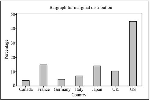
Interpretation: The maximum percentage of students belongs to US whereas the minimum percentage of the students belongs to Canada.

(c)

To determine

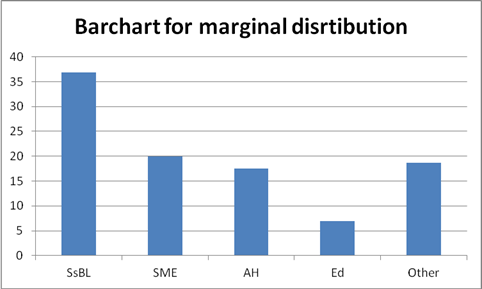
To find: The marginal distribution for the Field of study of the provided data and the graphical representation of the distribution.

Answer to Problem 153E

Solution: The obtained marginal totals are shown in the below table.

Field of study	SsBL	SME	AH	Ed	Other	Total
Marginal Percentage	36.888	19.908	17.504	6.971	18.728	100

And the graphical representation is shown below:

Explanation of Solution

Calculation: To obtained the marginal totals, below steps are followed in the Minitab software.

Step 1: Enter the data in Minitab worksheet.

Step 2: Go to Stat > Tables > Descriptive Statistics.

Step 3: Select “Field” in “For rows” and select “Country” in “For columns”. And select “Count” in “Frequencies are in”.

Step 4: Select the option “Total percents” and under the “Categorical Variables”.

Step 5: Click OK twice.

The percentage of totals are obtained as the Minitab output. The obtained marginal distribution are shown in the below table.

Field of study	SsBL	SME	AH	Ed	Other	Total
Marginal Percentage	17.504	6.971	18.728	19.908	36.888	100

Graph: The marginal distribution is graphically shown by using the bar graph. To obtain the graphical representation, below steps are followed in the Minitab software.

Step 1: Insert the data into the worksheet.

Step 2: Go to Graph $\to$ Bar Chart.

Step 3: Click on the drop down menu of “Bar represents” and select “Values from table”.

Step 3: Select “Simple” and click “OK”.

Step 4: Specify the “Graph variables” and “Categorical variable”.

Step 5: Click “OK”.

The bar graph is obtained as:

Interpretation: The maximum percentage of students studies SsBL fields whereas the minimum percentage of the students studies Ed.