Chapter 2.5, Problem 112E

(a)

To determine

To find: The predicted values and residuals for each of the four regression equation.

Answer to Problem 112E

Solution: The predicted values and residuals for Data set A is given below:

$x_A$	$y_A$	Predicted values	Residual
10	8.04	8.001	0.039
8	6.95	7.001	$-0.051$
13	7.58	9.501	$-1.921$
9	8.81	7.501	1.309
11	8.33	8.501	$-0.171$
14	9.96	10.001	$-0.041$
6	7.24	6.001	1.239
4	4.26	5.000	$-0.740$
12	10.84	9.001	1.839
7	4.82	6.501	$-1.681$
5	5.68	5.501	0.179

The predicted values and residuals for Data set B is given below:

$x_B$	$y_B$	Predicted values	Residual
10	9.14	8.001	1.139
8	8.14	7.001	1.139
13	8.74	9.501	$-0.761$
9	8.77	7.501	1.269
11	9.26	8.501	0.759
14	8.10	10.001	$-1.901$
6	6.13	6.001	0.129
4	3.10	5.000	$-1.901$
12	9.13	9.001	0.129
7	7.26	6.501	0.759
5	4.74	5.501	$-0.761$

The predicted values and residuals for Data set C is given below:

$x_C$	$y_C$	Predicted values	Residual
10	7.46	7.999	$-0.540$
8	6.77	7.000	$-0.230$
13	12.74	9.499	3.241
9	7.11	7.50	$-0.390$
11	7.81	8.499	$-0.689$
14	8.84	9.999	$-1.159$
6	6.08	6.001	0.079
4	5.39	5.001	0.389
12	8.15	8.999	$-0.849$
7	6.42	6.501	$-0.081$
5	5.73	5.501	0.229

The predicted values and residuals for Data set D is given below:

$x_D$	$y_D$	Predicted values	Residual
8	6.58	7.001	$-0.421$
8	5.76	7.001	$-1.241$
8	7.71	7.001	0.709
8	8.84	7.001	1.839
8	8.47	7.001	1.469
8	7.04	7.001	0.039
8	5.25	7.001	$-1.751$
8	5.56	7.001	$-1.441$
8	7.91	7.001	0.909
8	6.89	7.001	$-0.111$
19	12.50	12.5	$-0.000$

Explanation of Solution

Calculation: To predict y for Data set A, Minitab is used. The steps to be followed are:

Step 1: Go to the Minitab worksheet.

Step 2: Go to Stat > Regression > Regression.

Step 3: Enter the variable $y_A$ in the response and enter the variable $x_A$ in the predictor column.

Step 4: Go to results and select “The table of fits and residuals.”

Step 5: Click OK.

Hence, the result is

$x_A$	$y_A$	Predicted values	Residual
10	8.04	8.001	0.039
8	6.95	7.001	$-0.051$
13	7.58	9.501	$-1.921$
9	8.81	7.501	1.309
11	8.33	8.501	$-0.171$
14	9.96	10.001	$-0.041$
6	7.24	6.001	1.239
4	4.26	5.000	$-0.740$
12	10.84	9.001	1.839
7	4.82	6.501	$-1.681$
5	5.68	5.501	0.179

To predict y for Data set B, Minitab is used. The steps to be followed are:

Step 1: Go to the Minitab worksheet.

Step 2: Go to Stat > Regression > Regression.

Step 3: Enter the variable $y_B$ in the response and enter the variable $x_B$ in the predictor column.

Step 4: Go to results and select “The table of fits and residuals.”

Step 5: Click OK.

Hence, the result is

$x_B$	$y_B$	Predicted values	Residual
10	9.14	8.001	1.139
8	8.14	7.001	1.139
13	8.74	9.501	$-0.761$
9	8.77	7.501	1.269
11	9.26	8.501	0.759
14	8.10	10.001	$-1.901$
6	6.13	6.001	0.129
4	3.10	5.000	$-1.901$
12	9.13	9.001	0.129
7	7.26	6.501	0.759
5	4.74	5.501	$-0.761$

To predict y for Data set C, Minitab is used. The steps to be followed are:

Step 1: Go to the Minitab worksheet.

Step 2: Go to Stat > Regression > Regression.

Step 3: Enter the variable $y_C$ in the response and enter the variable $x_C$ in the predictor column.

Step 4: Go to results and select “The table of fits and residuals.”

Step 5: Click OK.

Hence, the result is

$x_C$	$y_C$	Predicted values	Residual
10	7.46	7.999	$-0.540$
8	6.77	7.000	$-0.230$
13	12.74	9.499	3.241
9	7.11	7.50	$-0.390$
11	7.81	8.499	$-0.689$
14	8.84	9.999	$-1.159$
6	6.08	6.001	0.079
4	5.39	5.001	0.389
12	8.15	8.999	$-0.849$
7	6.42	6.501	$-0.081$
5	5.73	5.501	0.229

To predict y for Data set D, Minitab is used. The steps to be followed are:

Step 1: Go to the Minitab worksheet.

Step 2: Go to Stat > Regression > Regression.

Step 3: Enter the variable $y_D$ in the response and enter the variable $x_D$ in the predictor column.

Step 4: Go to results and select “The table of fits and residuals.”

Step 5: Click OK.

Hence, the result is

$x_D$	$y_D$	Predicted values	Residual
8	6.58	7.001	$-0.421$
8	5.76	7.001	$-1.241$
8	7.71	7.001	0.709
8	8.84	7.001	1.839
8	8.47	7.001	1.469
8	7.04	7.001	0.039
8	5.25	7.001	$-1.751$
8	5.56	7.001	$-1.441$
8	7.91	7.001	0.909
8	6.89	7.001	$-0.111$
19	12.50	12.5	$-0.000$

Interpretation: The residual values are the differences of observed value and the predicted value.

(b)

To determine

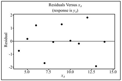
To graph: The residual versus x for each of the four datasets.

Explanation of Solution

Graph: To plot the residual versus x for each of the four datasets, Minitab is used. The steps to be followed are:

Step 1: Go to the Minitab worksheet.

Step 2: Go to Stat > Regression > Regression.

Step 3: Enter the variable $y_A$ in the response and enter the variable $x_A$ in the predictor column.

Step 4: Go to graph and select Residual versus fits.

Step 5: Click OK.

Hence, the obtained graph is

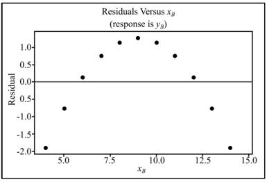
Similarly, repeat the steps for the residual plot versus x for Dataset B:

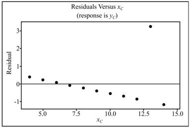
The residual plot versus x for Dataset C:

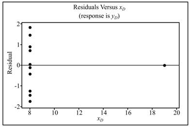
The residual plot versus x for Dataset D:

(c)

To determine

To explain: The summary for the residuals.

Answer to Problem 112E

Solution: The regression lines for datasets A and C fit the data quite well. The residual plot for dataset C shows strong correlation between the variables.

Explanation of Solution

For the Data set A, the residual plot has no correlation around a zero residual and this line fits the data quite well. For Data set B, the residual plot is in the form of arc and shows no correlation. This regression line is not a good representation of the data. For the Data set C, there is a strong correlation between the variables. So, the regression line fits well in the data and shows one outlier. For the Data set D, the residual plot is vertical. This is not a good prediction equation and there is one outlier.