Introduction to the Practice of Statistics
9th Edition
ISBN: 9781319013387
Author: David S. Moore, George P. McCabe, Bruce A. Craig
Publisher: W. H. Freeman
bartleby

Concept explainers

bartleby

Videos

Question
Book Icon
Chapter 2.5, Problem 96E

(a)

To determine

To find: The four residuals for the data provided on the counts over different times.

(a)

Expert Solution
Check Mark

Answer to Problem 96E

Solution: The residuals for the four counts are obtained as 49.9 _, 61.7_, 26.3_, and 38.1_.

Explanation of Solution

Calculation: The regression equation for the provided data set is as follows:

Count=602.8(74.7×Time)

Here, the response variable (represented as y) is ‘count,’ and the explanatory variable (represented as x) is ‘time.’ The estimated counts are obtained by substituting the respective values of time (1, 3, 5 and 7) in the regression equation.

For time x1=1, the value of count (represented as y^1 ) is calculated as follows:

Count=602.8(74.7×Time)=602.8(74.7×1)y^1=528.1

For time x2=3, the value of count (represented as y^2 ) is calculated as follows:

Count=602.8(74.7×Time)=602.8(74.7×3)y^2=378.7

For time x3=5, the value of count (represented as y^3 ) is calculated as follows:

count=602.8(74.7×time)=602.8(74.7×5)y^3=229.3

For time x4=7, the value of count (represented as y^4 ) is calculated as follows:

Count=602.8(74.7×Time)=602.8(74.7×7)y^4=79.9

The observed y values have been provided in the data and are written below:

y1=578y2=317y3=203y4=118

The residuals (represented as ei ) are the difference between the observed y values and predicted y values. The residuals for the above four observed and predicted values are calculated as follows:

For y1, the residual e1 is calculated as follows:

e1=Observed y1Predictedy1=y1y^1=578528.1=49.9

For y2, the residual e2 is calculated as follows:

e2=Observed y2Predictedy2=y2y^2=317378.7=61.7

For y3, the residual e3 is calculated as follows:

e3=Observed y3Predictedy3=y3y^3=203229.3=26.3

For y4, the residual e4 is calculated as follows:

e4=Observed y4Predictedy4=y4y^4=11879.9=38.1

Hence, the four residuals obtained are

e1=49.9 

e2=61.7

e3=26.3

e4=38.1

(b)

To determine

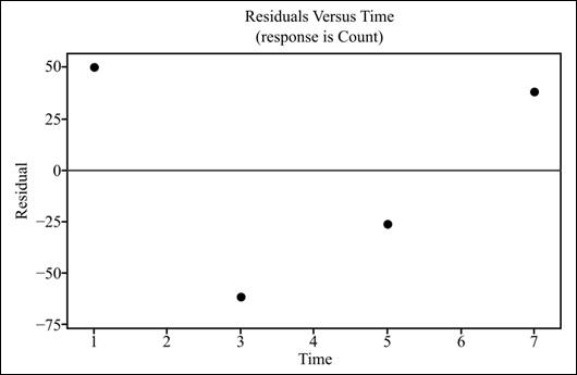
To graph: The model for residual versus time plot.

(b)

Expert Solution
Check Mark

Explanation of Solution

Graph: The residual versus time plot is obtained using the Minitab software by following the steps below:

Step 1: Enter the data in the Minitab worksheet.

Step 2: Go to Stat and select Regression and then select Regression again.

Step 3: Enter the response variable as ‘Count’ and Predictors as ‘Time.’

Step 4: Under Graphs option, choose Residuals versus order.

Step 5: Fill in Residual versus the variables as ‘Time.’

Step 6: Click on Ok.

The resultant graph is obtained as follows:

Introduction to the Practice of Statistics, Chapter 2.5, Problem 96E

(c)

To determine

To explain: Interpretation of the obtained residual plot.

(c)

Expert Solution
Check Mark

Answer to Problem 96E

Solution: Since there is no pattern observed in the residuals versus time plot, it can be concluded that the provided model is appropriate to estimate the count variable.

Explanation of Solution

The residual plot has no specific pattern. The plot seems to be scattered and nonlinear. The two residuals, e1 as 49.9  and e4 as 38.1, are positive, and the two residuals e2 as 61.7 and e3 as 26.3 are negative. This implies that the residuals are scattered above as well as below the x- axis. The uniform scattering of the residuals represents a good sign. Thus, it can be said that the provided regression model is suitable to predict the count variable.

Want to see more full solutions like this?

Subscribe now to access step-by-step solutions to millions of textbook problems written by subject matter experts!

Chapter 2 Solutions

Introduction to the Practice of Statistics

Ch. 2.2 - Prob. 11UYKCh. 2.2 - Prob. 12UYKCh. 2.2 - Prob. 13UYKCh. 2.2 - Prob. 14UYKCh. 2.2 - Prob. 15UYKCh. 2.2 - Prob. 16ECh. 2.2 - Prob. 17ECh. 2.2 - Prob. 18ECh. 2.2 - Prob. 19ECh. 2.2 - Prob. 20ECh. 2.2 - Prob. 21ECh. 2.2 - Prob. 22ECh. 2.2 - Prob. 23ECh. 2.2 - Prob. 24ECh. 2.2 - Prob. 25ECh. 2.2 - Prob. 26ECh. 2.2 - Prob. 27ECh. 2.2 - Prob. 28ECh. 2.2 - Prob. 29ECh. 2.2 - Prob. 30ECh. 2.2 - Prob. 31ECh. 2.2 - Prob. 32ECh. 2.2 - Prob. 33ECh. 2.2 - Prob. 34ECh. 2.2 - Prob. 35ECh. 2.2 - Prob. 36ECh. 2.2 - Prob. 37ECh. 2.3 - Prob. 38UYKCh. 2.3 - Prob. 39UYKCh. 2.3 - Prob. 40ECh. 2.3 - Prob. 41ECh. 2.3 - Prob. 42ECh. 2.3 - Prob. 43ECh. 2.3 - Prob. 44ECh. 2.3 - Prob. 45ECh. 2.3 - Prob. 46ECh. 2.3 - Prob. 47ECh. 2.3 - Prob. 48ECh. 2.3 - Prob. 49ECh. 2.3 - Prob. 50ECh. 2.3 - Prob. 51ECh. 2.3 - Prob. 52ECh. 2.3 - Prob. 53ECh. 2.3 - Prob. 54ECh. 2.3 - Prob. 55ECh. 2.3 - Prob. 56ECh. 2.3 - Prob. 57ECh. 2.3 - Prob. 58ECh. 2.3 - Prob. 59ECh. 2.3 - Prob. 60ECh. 2.4 - Prob. 61UYKCh. 2.4 - Prob. 62UYKCh. 2.4 - Prob. 63UYKCh. 2.4 - Prob. 64UYKCh. 2.4 - Prob. 65ECh. 2.4 - Prob. 66ECh. 2.4 - Prob. 67ECh. 2.4 - Prob. 68ECh. 2.4 - Prob. 69ECh. 2.4 - Prob. 70ECh. 2.4 - Prob. 71ECh. 2.4 - Prob. 72ECh. 2.4 - Prob. 73ECh. 2.4 - Prob. 74ECh. 2.4 - Prob. 75ECh. 2.4 - Prob. 76ECh. 2.4 - Prob. 77ECh. 2.4 - Prob. 78ECh. 2.4 - Prob. 79ECh. 2.4 - Prob. 80ECh. 2.4 - Prob. 81ECh. 2.4 - Prob. 82ECh. 2.4 - Prob. 83ECh. 2.4 - Prob. 84ECh. 2.4 - Prob. 85ECh. 2.4 - Prob. 86ECh. 2.4 - Prob. 87ECh. 2.4 - Prob. 88ECh. 2.4 - Prob. 89ECh. 2.4 - Prob. 90ECh. 2.4 - Prob. 91ECh. 2.5 - Prob. 92UYKCh. 2.5 - Prob. 93UYKCh. 2.5 - Prob. 94ECh. 2.5 - Prob. 95ECh. 2.5 - Prob. 96ECh. 2.5 - Prob. 97ECh. 2.5 - Prob. 98ECh. 2.5 - Prob. 99ECh. 2.5 - Prob. 100ECh. 2.5 - Prob. 101ECh. 2.5 - Prob. 102ECh. 2.5 - Prob. 103ECh. 2.5 - Prob. 104ECh. 2.5 - Prob. 105ECh. 2.5 - Prob. 106ECh. 2.5 - Prob. 107ECh. 2.5 - Prob. 108ECh. 2.5 - Prob. 110ECh. 2.5 - Prob. 111ECh. 2.5 - Prob. 112ECh. 2.6 - Prob. 113UYKCh. 2.6 - Prob. 114UYKCh. 2.6 - Prob. 115UYKCh. 2.6 - Prob. 116UYKCh. 2.6 - Prob. 117UYKCh. 2.6 - Prob. 118UYKCh. 2.6 - Prob. 119ECh. 2.6 - Prob. 120ECh. 2.6 - Prob. 121ECh. 2.6 - Prob. 122ECh. 2.6 - Prob. 123ECh. 2.6 - Prob. 124ECh. 2.6 - Prob. 125ECh. 2.6 - Prob. 126ECh. 2.6 - Prob. 127ECh. 2.6 - Prob. 128ECh. 2.6 - Prob. 129ECh. 2.6 - Prob. 130ECh. 2.7 - Prob. 131ECh. 2.7 - Prob. 132ECh. 2.7 - Prob. 133ECh. 2.7 - Prob. 134ECh. 2.7 - Prob. 135ECh. 2.7 - Prob. 136ECh. 2.7 - Prob. 137ECh. 2.7 - Prob. 138ECh. 2.7 - Prob. 139ECh. 2.7 - Prob. 140ECh. 2.7 - Prob. 141ECh. 2.7 - Prob. 142ECh. 2.7 - Prob. 143ECh. 2 - Prob. 144ECh. 2 - Prob. 145ECh. 2 - Prob. 146ECh. 2 - Prob. 147ECh. 2 - Prob. 148ECh. 2 - Prob. 149ECh. 2 - Prob. 150ECh. 2 - Prob. 151ECh. 2 - Prob. 152ECh. 2 - Prob. 153ECh. 2 - Prob. 154ECh. 2 - Prob. 155ECh. 2 - Prob. 156ECh. 2 - Prob. 157ECh. 2 - Prob. 158ECh. 2 - Prob. 159ECh. 2 - Prob. 160ECh. 2 - Prob. 161ECh. 2 - Prob. 162ECh. 2 - Prob. 163ECh. 2 - Prob. 164ECh. 2 - Prob. 165ECh. 2 - Prob. 166ECh. 2 - Prob. 167ECh. 2 - Prob. 168ECh. 2 - Prob. 169ECh. 2 - Prob. 170ECh. 2 - Prob. 171ECh. 2 - Prob. 172ECh. 2 - Prob. 173ECh. 2 - Prob. 174ECh. 2 - Prob. 175ECh. 2 - Prob. 176E
Knowledge Booster
Background pattern image
Statistics
Learn more about
Need a deep-dive on the concept behind this application? Look no further. Learn more about this topic, statistics and related others by exploring similar questions and additional content below.
Recommended textbooks for you
Text book image
MATLAB: An Introduction with Applications
Statistics
ISBN:9781119256830
Author:Amos Gilat
Publisher:John Wiley & Sons Inc
Text book image
Probability and Statistics for Engineering and th...
Statistics
ISBN:9781305251809
Author:Jay L. Devore
Publisher:Cengage Learning
Text book image
Statistics for The Behavioral Sciences (MindTap C...
Statistics
ISBN:9781305504912
Author:Frederick J Gravetter, Larry B. Wallnau
Publisher:Cengage Learning
Text book image
Elementary Statistics: Picturing the World (7th E...
Statistics
ISBN:9780134683416
Author:Ron Larson, Betsy Farber
Publisher:PEARSON
Text book image
The Basic Practice of Statistics
Statistics
ISBN:9781319042578
Author:David S. Moore, William I. Notz, Michael A. Fligner
Publisher:W. H. Freeman
Text book image
Introduction to the Practice of Statistics
Statistics
ISBN:9781319013387
Author:David S. Moore, George P. McCabe, Bruce A. Craig
Publisher:W. H. Freeman
Correlation Vs Regression: Difference Between them with definition & Comparison Chart; Author: Key Differences;https://www.youtube.com/watch?v=Ou2QGSJVd0U;License: Standard YouTube License, CC-BY
Correlation and Regression: Concepts with Illustrative examples; Author: LEARN & APPLY : Lean and Six Sigma;https://www.youtube.com/watch?v=xTpHD5WLuoA;License: Standard YouTube License, CC-BY