
Connect Hosted by ALEKS Online Access for Elementary Statistics
3rd Edition
ISBN: 9781260373769
Author: William Navidi
Publisher: MCGRAW-HILL HIGHER EDUCATION
expand_more
expand_more
format_list_bulleted
Videos
Textbook Question
Chapter 2.3, Problem 25E
Looking for a job: The following table presents the U.S. unemployment rate for each of the years 1993 through 2016.
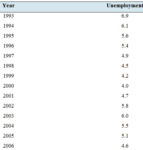
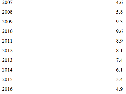
- Construct a time-series plot of the unemployment rate.
- For which periods of time was the unemployment rate increasing? For which periods was it decreasing?
Expert Solution & Answer
Want to see the full answer?
Check out a sample textbook solution
Students have asked these similar questions
The accompanying data represent health care expenditures per capita (per person) as a percentage of the U.S. gross domestic product (GDP) from 2007 to 2013. Gross domestic product is the total value of all goods and services created during the course
of the year Complete parts (a) through (c) below.
Click the icon to view the data table.
(a) Construct a time-series plot that a politician would create to support the position that health care expenditures are increasing and must be slowed. Choose the correct graph below
OD.
O C.
OB
OA
A
Q
A
Q
Q
25,000+
11,000
Q
Q
3
2
G
HIER
11200
2H
7,000++
C
2013
of
+
2013
2007
2007
Year
Year
Year
(b) Construct a time-series plot that the health care industry would create to refute the opinion of the politician. Choose the correct graph below.
OB.
O C.
O A.
A
Q
A
Q
11,000
Q
(C)
7,000+
201
20
7.000+++++++*
2007
2007
2013
2013
Year
Year
(c) Explain how different measures may be used to support two completely different positions. Choose the correct answer…
The following graph shows the annual number of car accidents in California. Which of the following
statements about the annual number of car accidents is an accurate conclusion?
Yearly Car Accidents
180,000
160,000
140,000
120,000
100,000
80,000
60,000
40,000
20,000
2000
2005
Year
1985
1990
1995
2010
2015
2020
e 2018 Glynlyon, Inc.
O There is a greater decrease in the annual number of car accidents from 1994 to 1995 than from 1997 to 1998.
O There is a smaller decrease in the annual number of car accidents from 1999 to 2000 than from 1997 to 1998.
O There is a smaller increase in the annualnumber of car accidents from 1995 to 1996 than from 1998 to 1999.
O There is a greater increase in the annual number of car accidents from 1993 to 1994 than from 1996 to 1997.
Car Accidents
Find the MSE in part (b) please.
Chapter 2 Solutions
Connect Hosted by ALEKS Online Access for Elementary Statistics
Ch. 2.1 - In Exercises 5-8, fill in each blank with the...Ch. 2.1 - In Exercises 5-8, fill in each blank with the...Ch. 2.1 - In Exercises 5-8, fill in each blank with the...Ch. 2.1 - In Exercises 5-8, fill in each blank with the...Ch. 2.1 - In Exercises 9—12, determine whether the...Ch. 2.1 - In Exercises 9—12, determine whether the...Ch. 2.1 - In Exercises 9—12, determine whether the...Ch. 2.1 - In Exercises 9—12, determine whether the...Ch. 2.1 - The following bar graph presents the average...Ch. 2.1 - The most common blood typing system divides human...
Ch. 2.1 - Following is a pie chart that presents the...Ch. 2.1 - Government spending: The following pie chart...Ch. 2.1 - U.S. population: The following side-by-side bar...Ch. 2.1 - Super Bowl: The following side-by-side bar graph...Ch. 2.1 - Smartphone sales: The following frequency...Ch. 2.1 - Popular video games: The following frequency...Ch. 2.1 - More smartphones: Using the data in Exercise 19:...Ch. 2.1 - More video games: Using the data in Exercise 20:...Ch. 2.1 - Hospital admissions: The following frequency...Ch. 2.1 - World population: Following are the populations of...Ch. 2.1 - Ages of video garners: The Nielsen Company...Ch. 2.1 - How secure is your job? In a survey, employed...Ch. 2.1 - Back up your data: In a survey commissioned by the...Ch. 2.1 - Education levels: The following frequency...Ch. 2.1 - Twitter followers: The following frequency...Ch. 2.1 - Music sales: The following frequency distribution...Ch. 2.1 - Keeping up with the Kardashians: The following...Ch. 2.1 - Bought a new car lately? The following table...Ch. 2.1 - Bought a new- truck lately? The following table...Ch. 2.1 - Happy Halloween: The following table presents...Ch. 2.1 - Native languages: The following frequency...Ch. 2.1 - Proportion of females: Following are the...Ch. 2.2 - Prob. 5ECh. 2.2 - In Exercises 5—8, fill in each blank with the...Ch. 2.2 - In Exercises 5—8, fill in each blank with the...Ch. 2.2 - In Exercises 5—8, fill in each blank with the...Ch. 2.2 - In Exercises 9—12, determine whether the...Ch. 2.2 - In Exercises 9—12, determine whether the...Ch. 2.2 - In Exercises 9—12, determine whether the...Ch. 2.2 - In Exercises 9—12, determine whether the...Ch. 2.2 - In Exercises 13—16, classify the histogram as...Ch. 2.2 - In Exercises 13—16, classify the histogram as...Ch. 2.2 - In Exercises 13—16, classify the histogram as...Ch. 2.2 - In Exercises 13—16, classify the histogram as...Ch. 2.2 - In Exercises 17 and 18, classify the histogram as...Ch. 2.2 - In Exercises 17 and 18, classify the histogram as...Ch. 2.2 - Student heights: The following frequency histogram...Ch. 2.2 - Trained rats: Forty rats were trained to run a...Ch. 2.2 - Cholesterol: The following histogram shows the...Ch. 2.2 - Blood pressure: The following histogram shows the...Ch. 2.2 - Olympic athletes: The following frequency...Ch. 2.2 - Hows the weather? The following relative frequency...Ch. 2.2 - Skewed which way? For which of the following data...Ch. 2.2 - Skewed which way? For which of the following data...Ch. 2.2 - Batting average: The following frequency...Ch. 2.2 - Batting average: The following frequency...Ch. 2.2 - Time spent playing video games: A sample of 200...Ch. 2.2 - Murder, she wrote: The following frequency...Ch. 2.2 - BMW prices: The following table presents the...Ch. 2.2 - Geysers: The geyser Old Faithful in Yellowstone...Ch. 2.2 - Hail to the chief: There have been 58 presidential...Ch. 2.2 - Internet radio: The following table presents the...Ch. 2.2 - Brothers and sisters: Thirty students in a...Ch. 2.2 - Cough, cough: The following table presents the...Ch. 2.2 - Prob. 37ECh. 2.2 - Prob. 38ECh. 2.2 - Prob. 39ECh. 2.2 - Prob. 40ECh. 2.2 - Frequency polygon: Using the data in Exercise 29:...Ch. 2.2 - Prob. 42ECh. 2.2 - Ogive: Using the data in Exercise 27: Compute the...Ch. 2.2 - Ogive: Using the data in Exercise 28: Compute the...Ch. 2.2 - Ogive: Using the data in Exercise 29: Compute the...Ch. 2.2 - Prob. 46ECh. 2.2 - Prob. 47ECh. 2.2 - Prob. 48ECh. 2.2 - Prob. 49ECh. 2.2 - Prob. 50ECh. 2.2 - Prob. 51ECh. 2.2 - Prob. 52ECh. 2.2 - Frequencies and relative frequencies: The...Ch. 2.3 - In Exercises 3—6, fill in each blank with the...Ch. 2.3 - In Exercises 3—6, fill in each blank with the...Ch. 2.3 - In Exercises 3—6, fill in each blank with the...Ch. 2.3 - In Exercises 3—6, fill in each blank with the...Ch. 2.3 - Prob. 7ECh. 2.3 - In Exercises 7—10, determine whether the...Ch. 2.3 - In Exercises 7—10, determine whether the...Ch. 2.3 - In Exercises 7—10, determine whether the...Ch. 2.3 - Construct a stem-and-leaf plot for the following...Ch. 2.3 - Construct a stem-and-leaf plot for the following...Ch. 2.3 - List the data in the following stem-and-leaf plot....Ch. 2.3 - List the data in the following stein-and-leaf...Ch. 2.3 - Construct a dotplot for the data in Exercise 11.Ch. 2.3 - Prob. 16ECh. 2.3 - BMW prices: The following table presents the...Ch. 2.3 - Hows the weather? The following table presents the...Ch. 2.3 - Air pollution: The following table presents...Ch. 2.3 - Technology salaries: The following table presents...Ch. 2.3 - Tennis and golf: Following are the ages of the...Ch. 2.3 - Pass the popcorn: Following are the running times...Ch. 2.3 - More weather: Construct a dotplot for the data in...Ch. 2.3 - Prob. 24ECh. 2.3 - Looking for a job: The following table presents...Ch. 2.3 - Prob. 26ECh. 2.3 - Military spending: The following table presents...Ch. 2.3 - Prob. 28ECh. 2.3 - Dining out: The following time-series plot...Ch. 2.3 - Prob. 30ECh. 2.3 - Prob. 31ECh. 2.3 - More gold: The following time series plot presents...Ch. 2.3 - Prob. 33ECh. 2.3 - Prob. 34ECh. 2.3 - Vote: The following time-series plot presents the...Ch. 2.3 - Arctic ice sheet: The following table presents the...Ch. 2.3 - Prob. 37ECh. 2.4 - In Exercises 3 and 4, fill in each blank with the...Ch. 2.4 - In Exercises 3 and 4, fill in each blank with the...Ch. 2.4 - CD sales decline: Sales of CDs have been declining...Ch. 2.4 - Music sales: The following time-series plot and...Ch. 2.4 - Stock market prices: The Dow Jones Industrial...Ch. 2.4 - Save your money: In 2007, U.S. residents saved...Ch. 2.4 - Ill take mine with mustard: The following bar...Ch. 2.4 - Stream or download? The following bar graph...Ch. 2.4 - Female senators: Of the 100 members of the United...Ch. 2.4 - Age at marriage: Data compiled by the U.S. Census...Ch. 2.4 - College degrees: Both of the following time-series...Ch. 2.4 - Food expenditures: Both of the following...Ch. 2.4 - Prob. 15ECh. 2 - Following is the list of letter grades for...Ch. 2 - Prob. 2CQCh. 2 - Construct a frequency bar graph for the data in...Ch. 2 - Prob. 4CQCh. 2 - Prob. 5CQCh. 2 - Prob. 6CQCh. 2 - Prob. 7CQCh. 2 - Prob. 8CQCh. 2 - Prob. 9CQCh. 2 - Prob. 10CQCh. 2 - Following are the prices (in dollars) for a sample...Ch. 2 - Prob. 12CQCh. 2 - Prob. 13CQCh. 2 - Prob. 14CQCh. 2 - Prob. 15CQCh. 2 - Trust your doctor: The General Social Survey...Ch. 2 - Internet browsers: The following relative...Ch. 2 - Prob. 3RECh. 2 - Prob. 4RECh. 2 - Prob. 5RECh. 2 - House freshmen: Newly elected members of the U.S....Ch. 2 - More freshmen: For the data in Exercise 6:...Ch. 2 - Royalty: Following are the ages at death for all...Ch. 2 - Prob. 9RECh. 2 - Prob. 10RECh. 2 - Prob. 11RECh. 2 - Prob. 12RECh. 2 - Prob. 13RECh. 2 - Prob. 14RECh. 2 - Prob. 15RECh. 2 - Explain why the frequency bar graph and the...Ch. 2 - Prob. 2WAICh. 2 - Prob. 3WAICh. 2 - Prob. 4WAICh. 2 - Prob. 5WAICh. 2 - In the chapter introduction, we presented gas...Ch. 2 - In the chapter introduction, we presented gas...Ch. 2 - In the chapter introduction, we presented gas...Ch. 2 - Prob. 4CSCh. 2 - In the chapter introduction, we presented gas...Ch. 2 - Prob. 6CSCh. 2 - In the chapter introduction, we presented gas...Ch. 2 - Prob. 8CSCh. 2 - In the chapter introduction, we presented gas...
Knowledge Booster


Learn more about
Need a deep-dive on the concept behind this application? Look no further. Learn more about this topic, statistics and related others by exploring similar questions and additional content below.Similar questions
- Table 3 gives the annual sales (in millions of dollars) of a product from 1998 to 20006. What was the average rate of change of annual sales (a) between 2001 and 2002, and (b) between 2001 and 2004?arrow_forwardThe US. import of wine (in hectoliters) for several years is given in Table 5. Determine whether the trend appearslinear. Ifso, and assuming the trend continues, in what year will imports exceed 12,000 hectoliters?arrow_forwardDVD Player sales The table shows the number of DVD play-ers sold in a small electronics store in the years 2003-2013. What was the average rate of change of sales between 2003 and 2013? Whatwas the average rate of change of sales between 2003 and 2004? What was the average rate of change of sales between 2004 and 2005? Between which two successive years did DVD player sales increase most quickly?arrow_forward
- Table 4 gives the population of a town (in thousand) from 2000 to 2008. What was the average rate of change of population (a) between 2002 and 2004, and (b) between 2002 and 2006?arrow_forwardDVD Player Sales The table shows the number of DVD players sold in a small electronics store in the years 2003-2013. Year DVD players sold 2003 495 2004 513 2005 410 2006 402 2007 520 2008 580 2009 631 2010 719 2011 624 2012 582 2013 635 aWhat was the average rate of change of sales between 2003 and 2013? bWhat was the average rate of change of sales between 2003 and 2004? cWhat was the average rate of change of sales between 2004 and 2005? dBetween which two successive years did DVD player sales increase most quickly? Decrease most quickly?arrow_forwardThe U.S. Census tracks the percentage of persons 25 years or older who are college graduates. That data forseveral years is given in Table 4[14]. Determine whether the trend appears linear. If so, and assuming the trendcontinues. in what year will the percentage exceed 35%?arrow_forward
- Hi, Could you please help me. I can't get on the X-axis the correct years to show up in minitab. Thank you!arrow_forwardWhat characteristics would you expect from a time series that describes the number of vehicles travelling through the road Gotthard tunnel each day from the 1st of January 1985 to the 1st of January 2000? Select one or more: O a. An yearly seasonal component. O b. Trying to do forecasting is pointless. O C. An increasing trend. O d. Some degree of noise. O e. A weekly seasonal component.arrow_forwardFigure 2 shows the presidential salary that each US President earned in his first year in office. Which US President earned the median inflation-adjusted salary? Woodrow Wilson Dwight Eisenhower Jimmy Carter Bill Clinton Joe Bidenarrow_forward
- The figure below is a time-series graph showing overall death rates (from all causes) in a country for 1900 to 2015. The spike in 1919 was due to a worldwide epidemic of influenza. Write a few sentences summarizing the overall trend, describing how much the death rate changed over this period of time and putting the 1919 spike into context in terms of its impact on the population. Death Rate per 1000 Population 20 15 10 5 L ul lu luulu l luulul 1900 1910 1920 1930 1940 1950 1960 1970 1980 1990 2000 2010 2020 Year Choose the correct answer below. O A. The death rates have increased by about 30% since the 1920s. The death rate during the influenza epidemic was about half of its current rate. O B. The death rates have decreased by about 50% since the 1920s. The death rate during the influenza epidemic was over four times its current rate. C. The death rates have decreased by about 50% since the 1920s. The death rate during the influenza epidemic was about half of its current rate. O D.…arrow_forwardIn retail, a store manager uses time series models to understand shopping trends. Review the scatter plot of the store’s sales from 2010 through 2021 to answer the questions. See attached as image. Here is the data for Fiscal Year and Sales: Fiscal Year Sales 2010 $260,123.00 2011 $256,853.00 2012 $274,366.00 2013 $290,525.00 2014 $322,318.00 2015 $380,921.00 2016 $541,925.00 2017 $909,050.00 2018 $1,817,521.00 2019 $3,206,564.00 2020 $4,921,005.00 2021 $5,686,338.00 Time series decomposition seeks to separate the time series (Y) into 4 components: trend (T), cycle (C), seasonal (S), and irregular (I). What is the difference between these components? The model can be additive or multiplicative. When do you use each? Review the scatter plot of the exponential trend of the time series data. Do you observe a trend? If so, what type of trend do you observe? What predictions might you make about the store’s annual sales over the next few years?arrow_forwardTime seriesarrow_forward
arrow_back_ios
SEE MORE QUESTIONS
arrow_forward_ios
Recommended textbooks for you
 Algebra and Trigonometry (MindTap Course List)AlgebraISBN:9781305071742Author:James Stewart, Lothar Redlin, Saleem WatsonPublisher:Cengage Learning
 College AlgebraAlgebraISBN:9781305115545Author:James Stewart, Lothar Redlin, Saleem WatsonPublisher:Cengage Learning
 Trigonometry (MindTap Course List)TrigonometryISBN:9781337278461Author:Ron LarsonPublisher:Cengage Learning
 College Algebra (MindTap Course List)AlgebraISBN:9781305652231Author:R. David Gustafson, Jeff HughesPublisher:Cengage Learning
Algebra and Trigonometry (MindTap Course List)
Algebra
ISBN:9781305071742
Author:James Stewart, Lothar Redlin, Saleem Watson
Publisher:Cengage Learning
College Algebra
Algebra
ISBN:9781305115545
Author:James Stewart, Lothar Redlin, Saleem Watson
Publisher:Cengage Learning
Trigonometry (MindTap Course List)
Trigonometry
ISBN:9781337278461
Author:Ron Larson
Publisher:Cengage Learning
College Algebra (MindTap Course List)
Algebra
ISBN:9781305652231
Author:R. David Gustafson, Jeff Hughes
Publisher:Cengage Learning
Time Series Analysis Theory & Uni-variate Forecasting Techniques; Author: Analytics University;https://www.youtube.com/watch?v=_X5q9FYLGxM;License: Standard YouTube License, CC-BY
Operations management 101: Time-series, forecasting introduction; Author: Brandoz Foltz;https://www.youtube.com/watch?v=EaqZP36ool8;License: Standard YouTube License, CC-BY