
Connect Hosted by ALEKS Online Access for Elementary Statistics
3rd Edition
ISBN: 9781260373769
Author: William Navidi
Publisher: MCGRAW-HILL HIGHER EDUCATION
expand_more
expand_more
format_list_bulleted
Concept explainers
Videos
Textbook Question
Chapter 2.4, Problem 12E
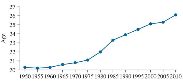
Age at marriage: Data compiled by the U.S. Census Bureau suggests that the age at which women first marry has increased over time. The following time-series plot presents the average age at which women first marry for the years 1950—2010. Does the plot present an accurate picture of the increase, or is it misleading? Explain.
Expert Solution & Answer
Want to see the full answer?
Check out a sample textbook solution
Students have asked these similar questions
The accompanying data represent health care expenditures per capita (per person) as a percentage of the U.S. gross domestic product (GDP) from 2007 to 2013. Gross domestic product is the total value of all goods and services created during the course
of the year Complete parts (a) through (c) below.
Click the icon to view the data table.
(a) Construct a time-series plot that a politician would create to support the position that health care expenditures are increasing and must be slowed. Choose the correct graph below
OD.
O C.
OB
OA
A
Q
A
Q
Q
25,000+
11,000
Q
Q
3
2
G
HIER
11200
2H
7,000++
C
2013
of
+
2013
2007
2007
Year
Year
Year
(b) Construct a time-series plot that the health care industry would create to refute the opinion of the politician. Choose the correct graph below.
OB.
O C.
O A.
A
Q
A
Q
11,000
Q
(C)
7,000+
201
20
7.000+++++++*
2007
2007
2013
2013
Year
Year
(c) Explain how different measures may be used to support two completely different positions. Choose the correct answer…
Can someone explain this from a mathematical perspective? Find a relation between the fraction of islands occupied by a species and time. There is a fixed number of islands. The distribution of the species across all islands is maintained by a balance between local extinctions and local colonization events.
The file P02_26.xlsx lists sales (in millions of dollars) of Dell Computer during the period 1987–1997 (where year 1 corresponds to 1987).
Year
Sales
1
69
2
159
3
258
4
389
5
546
6
890
7
2014
8
2873
9
3475
10
5296
11
7759
a. Fit a power and an exponential trend curve to these data. Which fits the data better?
b. Use your part a answer to predict 1999 sales for Dell.
c. Use your part a answer to describe how the sales of Dell have grown from year to year.
Chapter 2 Solutions
Connect Hosted by ALEKS Online Access for Elementary Statistics
Ch. 2.1 - In Exercises 5-8, fill in each blank with the...Ch. 2.1 - In Exercises 5-8, fill in each blank with the...Ch. 2.1 - In Exercises 5-8, fill in each blank with the...Ch. 2.1 - In Exercises 5-8, fill in each blank with the...Ch. 2.1 - In Exercises 9—12, determine whether the...Ch. 2.1 - In Exercises 9—12, determine whether the...Ch. 2.1 - In Exercises 9—12, determine whether the...Ch. 2.1 - In Exercises 9—12, determine whether the...Ch. 2.1 - The following bar graph presents the average...Ch. 2.1 - The most common blood typing system divides human...
Ch. 2.1 - Following is a pie chart that presents the...Ch. 2.1 - Government spending: The following pie chart...Ch. 2.1 - U.S. population: The following side-by-side bar...Ch. 2.1 - Super Bowl: The following side-by-side bar graph...Ch. 2.1 - Smartphone sales: The following frequency...Ch. 2.1 - Popular video games: The following frequency...Ch. 2.1 - More smartphones: Using the data in Exercise 19:...Ch. 2.1 - More video games: Using the data in Exercise 20:...Ch. 2.1 - Hospital admissions: The following frequency...Ch. 2.1 - World population: Following are the populations of...Ch. 2.1 - Ages of video garners: The Nielsen Company...Ch. 2.1 - How secure is your job? In a survey, employed...Ch. 2.1 - Back up your data: In a survey commissioned by the...Ch. 2.1 - Education levels: The following frequency...Ch. 2.1 - Twitter followers: The following frequency...Ch. 2.1 - Music sales: The following frequency distribution...Ch. 2.1 - Keeping up with the Kardashians: The following...Ch. 2.1 - Bought a new car lately? The following table...Ch. 2.1 - Bought a new- truck lately? The following table...Ch. 2.1 - Happy Halloween: The following table presents...Ch. 2.1 - Native languages: The following frequency...Ch. 2.1 - Proportion of females: Following are the...Ch. 2.2 - Prob. 5ECh. 2.2 - In Exercises 5—8, fill in each blank with the...Ch. 2.2 - In Exercises 5—8, fill in each blank with the...Ch. 2.2 - In Exercises 5—8, fill in each blank with the...Ch. 2.2 - In Exercises 9—12, determine whether the...Ch. 2.2 - In Exercises 9—12, determine whether the...Ch. 2.2 - In Exercises 9—12, determine whether the...Ch. 2.2 - In Exercises 9—12, determine whether the...Ch. 2.2 - In Exercises 13—16, classify the histogram as...Ch. 2.2 - In Exercises 13—16, classify the histogram as...Ch. 2.2 - In Exercises 13—16, classify the histogram as...Ch. 2.2 - In Exercises 13—16, classify the histogram as...Ch. 2.2 - In Exercises 17 and 18, classify the histogram as...Ch. 2.2 - In Exercises 17 and 18, classify the histogram as...Ch. 2.2 - Student heights: The following frequency histogram...Ch. 2.2 - Trained rats: Forty rats were trained to run a...Ch. 2.2 - Cholesterol: The following histogram shows the...Ch. 2.2 - Blood pressure: The following histogram shows the...Ch. 2.2 - Olympic athletes: The following frequency...Ch. 2.2 - Hows the weather? The following relative frequency...Ch. 2.2 - Skewed which way? For which of the following data...Ch. 2.2 - Skewed which way? For which of the following data...Ch. 2.2 - Batting average: The following frequency...Ch. 2.2 - Batting average: The following frequency...Ch. 2.2 - Time spent playing video games: A sample of 200...Ch. 2.2 - Murder, she wrote: The following frequency...Ch. 2.2 - BMW prices: The following table presents the...Ch. 2.2 - Geysers: The geyser Old Faithful in Yellowstone...Ch. 2.2 - Hail to the chief: There have been 58 presidential...Ch. 2.2 - Internet radio: The following table presents the...Ch. 2.2 - Brothers and sisters: Thirty students in a...Ch. 2.2 - Cough, cough: The following table presents the...Ch. 2.2 - Prob. 37ECh. 2.2 - Prob. 38ECh. 2.2 - Prob. 39ECh. 2.2 - Prob. 40ECh. 2.2 - Frequency polygon: Using the data in Exercise 29:...Ch. 2.2 - Prob. 42ECh. 2.2 - Ogive: Using the data in Exercise 27: Compute the...Ch. 2.2 - Ogive: Using the data in Exercise 28: Compute the...Ch. 2.2 - Ogive: Using the data in Exercise 29: Compute the...Ch. 2.2 - Prob. 46ECh. 2.2 - Prob. 47ECh. 2.2 - Prob. 48ECh. 2.2 - Prob. 49ECh. 2.2 - Prob. 50ECh. 2.2 - Prob. 51ECh. 2.2 - Prob. 52ECh. 2.2 - Frequencies and relative frequencies: The...Ch. 2.3 - In Exercises 3—6, fill in each blank with the...Ch. 2.3 - In Exercises 3—6, fill in each blank with the...Ch. 2.3 - In Exercises 3—6, fill in each blank with the...Ch. 2.3 - In Exercises 3—6, fill in each blank with the...Ch. 2.3 - Prob. 7ECh. 2.3 - In Exercises 7—10, determine whether the...Ch. 2.3 - In Exercises 7—10, determine whether the...Ch. 2.3 - In Exercises 7—10, determine whether the...Ch. 2.3 - Construct a stem-and-leaf plot for the following...Ch. 2.3 - Construct a stem-and-leaf plot for the following...Ch. 2.3 - List the data in the following stem-and-leaf plot....Ch. 2.3 - List the data in the following stein-and-leaf...Ch. 2.3 - Construct a dotplot for the data in Exercise 11.Ch. 2.3 - Prob. 16ECh. 2.3 - BMW prices: The following table presents the...Ch. 2.3 - Hows the weather? The following table presents the...Ch. 2.3 - Air pollution: The following table presents...Ch. 2.3 - Technology salaries: The following table presents...Ch. 2.3 - Tennis and golf: Following are the ages of the...Ch. 2.3 - Pass the popcorn: Following are the running times...Ch. 2.3 - More weather: Construct a dotplot for the data in...Ch. 2.3 - Prob. 24ECh. 2.3 - Looking for a job: The following table presents...Ch. 2.3 - Prob. 26ECh. 2.3 - Military spending: The following table presents...Ch. 2.3 - Prob. 28ECh. 2.3 - Dining out: The following time-series plot...Ch. 2.3 - Prob. 30ECh. 2.3 - Prob. 31ECh. 2.3 - More gold: The following time series plot presents...Ch. 2.3 - Prob. 33ECh. 2.3 - Prob. 34ECh. 2.3 - Vote: The following time-series plot presents the...Ch. 2.3 - Arctic ice sheet: The following table presents the...Ch. 2.3 - Prob. 37ECh. 2.4 - In Exercises 3 and 4, fill in each blank with the...Ch. 2.4 - In Exercises 3 and 4, fill in each blank with the...Ch. 2.4 - CD sales decline: Sales of CDs have been declining...Ch. 2.4 - Music sales: The following time-series plot and...Ch. 2.4 - Stock market prices: The Dow Jones Industrial...Ch. 2.4 - Save your money: In 2007, U.S. residents saved...Ch. 2.4 - Ill take mine with mustard: The following bar...Ch. 2.4 - Stream or download? The following bar graph...Ch. 2.4 - Female senators: Of the 100 members of the United...Ch. 2.4 - Age at marriage: Data compiled by the U.S. Census...Ch. 2.4 - College degrees: Both of the following time-series...Ch. 2.4 - Food expenditures: Both of the following...Ch. 2.4 - Prob. 15ECh. 2 - Following is the list of letter grades for...Ch. 2 - Prob. 2CQCh. 2 - Construct a frequency bar graph for the data in...Ch. 2 - Prob. 4CQCh. 2 - Prob. 5CQCh. 2 - Prob. 6CQCh. 2 - Prob. 7CQCh. 2 - Prob. 8CQCh. 2 - Prob. 9CQCh. 2 - Prob. 10CQCh. 2 - Following are the prices (in dollars) for a sample...Ch. 2 - Prob. 12CQCh. 2 - Prob. 13CQCh. 2 - Prob. 14CQCh. 2 - Prob. 15CQCh. 2 - Trust your doctor: The General Social Survey...Ch. 2 - Internet browsers: The following relative...Ch. 2 - Prob. 3RECh. 2 - Prob. 4RECh. 2 - Prob. 5RECh. 2 - House freshmen: Newly elected members of the U.S....Ch. 2 - More freshmen: For the data in Exercise 6:...Ch. 2 - Royalty: Following are the ages at death for all...Ch. 2 - Prob. 9RECh. 2 - Prob. 10RECh. 2 - Prob. 11RECh. 2 - Prob. 12RECh. 2 - Prob. 13RECh. 2 - Prob. 14RECh. 2 - Prob. 15RECh. 2 - Explain why the frequency bar graph and the...Ch. 2 - Prob. 2WAICh. 2 - Prob. 3WAICh. 2 - Prob. 4WAICh. 2 - Prob. 5WAICh. 2 - In the chapter introduction, we presented gas...Ch. 2 - In the chapter introduction, we presented gas...Ch. 2 - In the chapter introduction, we presented gas...Ch. 2 - Prob. 4CSCh. 2 - In the chapter introduction, we presented gas...Ch. 2 - Prob. 6CSCh. 2 - In the chapter introduction, we presented gas...Ch. 2 - Prob. 8CSCh. 2 - In the chapter introduction, we presented gas...
Knowledge Booster


Learn more about
Need a deep-dive on the concept behind this application? Look no further. Learn more about this topic, statistics and related others by exploring similar questions and additional content below.Similar questions
- Table 6 shows the year and the number ofpeople unemployed in a particular city for several years. Determine whether the trend appears linear. If so, and assuming the trend continues, in what year will the number of unemployed reach 5 people?arrow_forwardThe US. import of wine (in hectoliters) for several years is given in Table 5. Determine whether the trend appearslinear. Ifso, and assuming the trend continues, in what year will imports exceed 12,000 hectoliters?arrow_forwardWhat does the y -intercept on the graph of a logistic equation correspond to for a population modeled by that equation?arrow_forward
- The U.S. Census tracks the percentage of persons 25 years or older who are college graduates. That data forseveral years is given in Table 4[14]. Determine whether the trend appears linear. If so, and assuming the trendcontinues. in what year will the percentage exceed 35%?arrow_forwardTable 3 gives the annual sales (in millions of dollars) of a product from 1998 to 20006. What was the average rate of change of annual sales (a) between 2001 and 2002, and (b) between 2001 and 2004?arrow_forward6 This table shows the number of subscribers to a video streaming service in the first six years after it was founded. Year 2016 2017 2018 2019 2020 2021 Subscribers 182,000 304,000 433,000 669,000 1,027,000 1,356,000 What was the average rate of change in the number of subscribers between 2017 and 2020?arrow_forward
- The following graph shows the annual number of car accidents in California. Which of the following statements about the annual number of car accidents is an accurate conclusion? Yearly Car Accidents 180,000 160,000 140,000 120,000 100,000 80,000 60,000 40,000 20,000 2000 2005 Year 1985 1990 1995 2010 2015 2020 e 2018 Glynlyon, Inc. O There is a greater decrease in the annual number of car accidents from 1994 to 1995 than from 1997 to 1998. O There is a smaller decrease in the annual number of car accidents from 1999 to 2000 than from 1997 to 1998. O There is a smaller increase in the annualnumber of car accidents from 1995 to 1996 than from 1998 to 1999. O There is a greater increase in the annual number of car accidents from 1993 to 1994 than from 1996 to 1997. Car Accidentsarrow_forwardWith the growth of internet service providers, a researcher decides to examine whether there is a correlation between cost of internet service per month (rounded to the nearest peso) and degree of customer satisfaction (on a scale of 10 - 100 with a 10 being not at all satisfied and a 100 being extremely satisfied). The researcher only includes programs with comparable types of services. A sample of the data is provided below. d. Using your equation, estimate the satisfaction of the customer if the cost is P1175 per month. Ans = Blank 5 e. Using your equation, estimate the satisfaction of the customer if the cost is P245 per month. Ans = Blank 6arrow_forwardThe following table gives the average monthly exchange rate between the U.S. dollar and the euro for 2009. It shows that 1 euro was equivalent to 1.289 U.S. dollars in January 2009. Develop a trend line that could be used to predict the exchange rate for 2010. Use this model to predict the exchange rate for January 2010 and February 2010. MONTH ______________________ EXCHANGE RATE January ....................................... 1.289 February ...................................... 1.324 March ......................................... 1.321 April .......................................... 1.317 May ........................................... 1.280 June ........................................... 1.254 July ........................................... 1.230 August ....................................... 1.240 September ................................... 1.287 October ..................................... 1.298 November .................................. 1.283 December…arrow_forward
- Find the MSE in part (b) please.arrow_forwardTable 1: Which set of data would best be modeled by an exponential function? Y1 Y1 C X I Y1 Y1 2 3.5 14 42.5 98 189.5 2 3. Ч.5 6.75 10.125 15.188 2 3.5 8. 15.5 26 39.5 1 3.5 6.5 8. 9.5 4 4 4 123T5 123T5narrow_forwardIn retail, a store manager uses time series models to understand shopping trends. Review the scatter plot of the store’s sales from 2010 through 2021 to answer the questions. See attached as image. Here is the data for Fiscal Year and Sales: Fiscal Year Sales 2010 $260,123.00 2011 $256,853.00 2012 $274,366.00 2013 $290,525.00 2014 $322,318.00 2015 $380,921.00 2016 $541,925.00 2017 $909,050.00 2018 $1,817,521.00 2019 $3,206,564.00 2020 $4,921,005.00 2021 $5,686,338.00 Time series decomposition seeks to separate the time series (Y) into 4 components: trend (T), cycle (C), seasonal (S), and irregular (I). What is the difference between these components? The model can be additive or multiplicative. When do you use each? Review the scatter plot of the exponential trend of the time series data. Do you observe a trend? If so, what type of trend do you observe? What predictions might you make about the store’s annual sales over the next few years?arrow_forward
arrow_back_ios
SEE MORE QUESTIONS
arrow_forward_ios
Recommended textbooks for you

 Glencoe Algebra 1, Student Edition, 9780079039897...AlgebraISBN:9780079039897Author:CarterPublisher:McGraw Hill
Glencoe Algebra 1, Student Edition, 9780079039897...
Algebra
ISBN:9780079039897
Author:Carter
Publisher:McGraw Hill
Which is the best chart: Selecting among 14 types of charts Part II; Author: 365 Data Science;https://www.youtube.com/watch?v=qGaIB-bRn-A;License: Standard YouTube License, CC-BY