
ELEM. STATISTICS TEXT W/ MANUAL+CONNECT
1st Edition
ISBN: 9781260722031
Author: Navidi
Publisher: McGraw-Hill Publishing Co.
expand_more
expand_more
format_list_bulleted
Concept explainers
Videos
Textbook Question
Chapter 4.1, Problem 36E
Mortgage payments: The following table presents monthly interest rates, in percent, for 30-year and 15-year fixed-rate mortgages, for a recent year.
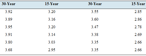
- Construct a
scatterplot of the 15-year rate (y) versus the 30-year rate (x). - Compute the
correlation coefficient between 30-year and 15-year rates. - When the 30-year rate is below average, would you expect the 15-year rate to be above or below average? Explain.
- Which of the following is the best interpretation of the correlation coefficient?
- When a bank increases the 30-year rate: that causes the 15-year rate to rise as well.
- Interest rates are determined by economic conditions. economic conditions cause 30-year rates to these same conditions cause 15 -year rates to increase as well.
- When a bank increases the 15-year rate, that causes the 30-year rate to rise as well.
Expert Solution & Answer
Want to see the full answer?
Check out a sample textbook solution
Students have asked these similar questions
Kim is interested in studying the relationship between mortgage rates and median
home prices. The data is provided below
Year Interest Rate (%) Median home price
1988 10.30 $183,800
1989 10.30 $183,200
1990 10.10 $174,900
1991 9.30 $173,500
1992 8.40 $172,900
1993 7.30 $173,200
1994 8.40 $173,200
1995 7.90 $169,700
1996 7.60 $174,500
1997 7.60 $177,900
1998 6.90 $188,100
1999 7.40 $203,200
2000 8.10 $230,200
2001 7.00 $258,200
2002 6.50 $309,800
2003 5.80 $329,800
2004 5.80…
How strong is the correlation between the inflation rate and 30-year treasury yields? The following data published by Fuji Securities are given as pairs of inflation rates and treasury yields for selected years over a 35-year period.
Inflation Rate
30-Year Treasure Yield
1.57%
3.10%
2.23
3.93
2.19
4.68
4.53
6.57
7.25
8.27
9.25
11.93
5.02
10.27
4.62
8.45
Compute the Pearson product-moment correlation coefficient to determine the strength of the correlation between these two variables. Comment on the strength and direction of the correlation.
(Round the intermediate values to 4 decimal places. Round your answer to 3 decimal places.)
a r= ?
b There is a strong negative relationship or strong positive relationship between the inflation rate and the thirty-year treasury yield. ?
Chapter 4 Solutions
ELEM. STATISTICS TEXT W/ MANUAL+CONNECT
Ch. 4.1 - In Exercises 9-12, fill in each blank with the...Ch. 4.1 - In Exercises 9-12, fill in each blank with the...Ch. 4.1 - In Exercises 9-12, fill in each blank with the...Ch. 4.1 - In Exercises 9-12, fill in each blank with the...Ch. 4.1 - Prob. 13ECh. 4.1 - Prob. 14ECh. 4.1 - In Exercises 13-16, determine whether the...Ch. 4.1 - In Exercises 13-16, determine whether the...Ch. 4.1 - In Exercises 17-20, compute the correlation...Ch. 4.1 - In Exercises 17-20, compute the correlation...
Ch. 4.1 - In Exercises 17-20, compute the correlation...Ch. 4.1 - In Exercises 17-20, compute the correlation...Ch. 4.1 - In Exercises 21-24, determine whether the...Ch. 4.1 - In Exercises 21-24, determine whether the...Ch. 4.1 - In Exercises 21-24, determine whether the...Ch. 4.1 - In Exercises 21-24, determine whether the...Ch. 4.1 - In Exercises 25-30, determine whether the...Ch. 4.1 - In Exercises 25-30, determine whether the...Ch. 4.1 - In Exercises 25-30, determine whether the...Ch. 4.1 - In Exercises 25-30, determine whether the...Ch. 4.1 - In Exercises 25-30, determine whether the...Ch. 4.1 - In Exercises 25-30, determine whether the...Ch. 4.1 - Price of eggs and milk: The following table...Ch. 4.1 - Government funding: The following table presents...Ch. 4.1 - Pass the ball: The following table lists the...Ch. 4.1 - Carbon footprint: Carbon dioxide (CO2) is produced...Ch. 4.1 - Foot temperatures: Foot ulcers are a common...Ch. 4.1 - Mortgage payments: The following table presents...Ch. 4.1 - Blood pressure: A blood pressure measurement...Ch. 4.1 - Prob. 38ECh. 4.1 - Police and crime: In a survey of cities in the...Ch. 4.1 - Age and education: A survey of U.S. adults showed...Ch. 4.1 - Whats the correlation? In a sample of adults, the...Ch. 4.1 - Prob. 42ECh. 4.1 - Changing means and standard deviations: A small...Ch. 4.2 - In Exercises 5-7, fill in each blank with the...Ch. 4.2 - In Exercises 5-7, fill in each blank with the...Ch. 4.2 - In Exercises 5-7, fill in each blank with the...Ch. 4.2 - Prob. 8ECh. 4.2 - Prob. 9ECh. 4.2 - Prob. 10ECh. 4.2 - Prob. 11ECh. 4.2 - Prob. 12ECh. 4.2 - In Exercises 13-16, compute the least-squares...Ch. 4.2 - In Exercises 13-16, compute the least-squares...Ch. 4.2 - In Exercises 13-16, compute the least-squares...Ch. 4.2 - In Exercises 13-16, compute the least-squares...Ch. 4.2 - Compute the least-squares regression he for...Ch. 4.2 - Compute the least-squares regression he for...Ch. 4.2 - In a hypothetical study of the relationship...Ch. 4.2 - Assume in a study of educational level in years...Ch. 4.2 - Price of eggs and milk: The following table...Ch. 4.2 - Government funding: The following table presents...Ch. 4.2 - Pass the ball: The following table lists the...Ch. 4.2 - Carbon footprint: Carbon dioxide (CO2) is produced...Ch. 4.2 - Foot temperatures: Foot ulcers are a common...Ch. 4.2 - Mortgage payments: The following table presents...Ch. 4.2 - Blood pressure: A blood pressure measurement...Ch. 4.2 - Butterfly wings: Do larger butterflies live...Ch. 4.2 - Interpreting technology: The following display...Ch. 4.2 - Interpreting technology: The following display...Ch. 4.2 - Interpreting technology: The following MINITAB...Ch. 4.2 - Interpreting technology: The following MINITAB...Ch. 4.2 - Prob. 33ECh. 4.2 - Prob. 34ECh. 4.2 - Least-squares regression line for z-scores: The...Ch. 4.3 - In Exercises 5-10, fill in each blank with the...Ch. 4.3 - In Exercises 5-10, fill in each blank with the...Ch. 4.3 - In Exercises 5-10, fill in each blank with the...Ch. 4.3 - In Exercises 5-10, fill in each blank with the...Ch. 4.3 - In Exercises 5-10, fill in each blank with the...Ch. 4.3 - Prob. 10ECh. 4.3 - Prob. 11ECh. 4.3 - In Exercises 11-14, determine whether the...Ch. 4.3 - Prob. 13ECh. 4.3 - In Exercises 11-14, determine whether the...Ch. 4.3 - For the following data set: Compute the...Ch. 4.3 - For the following data set: Compute the...Ch. 4.3 - For the following data set: Compute the...Ch. 4.3 - For the following data set: Compute the...Ch. 4.3 - Prob. 19ECh. 4.3 - Prob. 20ECh. 4.3 - Prob. 21ECh. 4.3 - Prob. 22ECh. 4.3 - Hot enough for you? The following table presents...Ch. 4.3 - Presidents and first ladies: The presents the ages...Ch. 4.3 - Mutant genes: In a study to determine whether the...Ch. 4.3 - Imports and exports: The following table presents...Ch. 4.3 - Energy consumption: The following table presents...Ch. 4.3 - Cost of health care: The following table presents...Ch. 4.3 - Prob. 29ECh. 4.3 - Prob. 30ECh. 4.3 - Prob. 31ECh. 4.3 - Transforming a variable: The following table...Ch. 4.3 - Prob. 33ECh. 4.3 - Prob. 34ECh. 4 - Compute the correlation coefficient for the...Ch. 4 - The number of theaters showing the movie Monsters...Ch. 4 - Use the data in Exercise 2 to compute the...Ch. 4 - A scatterplot has a correlation of r=1. Describe...Ch. 4 - Prob. 5CQCh. 4 - Prob. 6CQCh. 4 - Use the least-squares regression line computed in...Ch. 4 - Use the least-squares regression line computed in...Ch. 4 - Prob. 9CQCh. 4 - A scatterplot has a least-squares regression line...Ch. 4 - Prob. 11CQCh. 4 - Prob. 12CQCh. 4 - A sample of students was studied to determine the...Ch. 4 - In a scatter-plot; the point (-2, 7) is...Ch. 4 - The correlation coefficient for a data set is...Ch. 4 - Prob. 1RECh. 4 - Prob. 2RECh. 4 - Hows your mileage? Weight (in tons) and fuel...Ch. 4 - Prob. 4RECh. 4 - Energy efficiency: A sample of 10 households was...Ch. 4 - Energy efficiency: Using the data in Exercise 5:...Ch. 4 - Prob. 7RECh. 4 - Prob. 8RECh. 4 - Prob. 9RECh. 4 - Prob. 10RECh. 4 - Baby weights: The average gestational age (time...Ch. 4 - Commute times: Every morning, Tania leaves for...Ch. 4 - Prob. 13RECh. 4 - Prob. 14RECh. 4 - Prob. 15RECh. 4 - Describe an example which two variables are...Ch. 4 - Two variables x and y have a positive association...Ch. 4 - Prob. 3WAICh. 4 - Prob. 4WAICh. 4 - Prob. 5WAICh. 4 - Prob. 6WAICh. 4 - Prob. 7WAICh. 4 - Prob. 8WAICh. 4 - Prob. 9WAICh. 4 - The following table, reproduced from the chapter...Ch. 4 - Prob. 2CSCh. 4 - Prob. 3CSCh. 4 - Prob. 4CSCh. 4 - Prob. 5CSCh. 4 - Prob. 6CSCh. 4 - Prob. 7CSCh. 4 - Prob. 8CSCh. 4 - Prob. 9CSCh. 4 - Prob. 10CSCh. 4 - Prob. 11CSCh. 4 - Prob. 12CSCh. 4 - Prob. 13CSCh. 4 - If we are going to use data from this year to...Ch. 4 - Prob. 15CS
Knowledge Booster


Learn more about
Need a deep-dive on the concept behind this application? Look no further. Learn more about this topic, statistics and related others by exploring similar questions and additional content below.Similar questions
- An auctioneer of antique Iranian rugs kept records of his weekly auctions in order to determine the relationships among price, age of carpet or rug, number of people attending the auction, and the number of times the winning bidder had previously attended his auctions. He felt that, with this information, he could plan his auctions better, serve his steady customers better, and make a higher overall profit for himself. The results shown in the accompanying table were obtained.arrow_forwardAfter its move in 1990 to La Junta, Colorado, and its new initiatives, the DeBourgh Manufacturing Company began an upward climb of record sales. Suppose the figures shown here are the DeBourgh monthly sales figures from January 2001 through December 2009 (in $1,000s). a) Produce a time series plot. Are there any trends evident in the data? Does DeBourgh have a seasonal component to its sales? b) Deseasonalize the data using Multiplicative model with a 0.5 weighted moving average. Produce a time series plot of the deseasonalized data and add a trendline. c) Forecast the sales from January to December of the year 2010. d) Include a discussion of the general direction of sales and any seasonal tendencies that might be occurrinG Month 2001 2002 2003 2004 2005 2006 2007 2008 2009 January 139.7 165.1 177.8 228.6 266.7 431.8 381 431.8 495.3 February 114.3 177.8 203.2 254 317.5 457.2 406.4 444.5 533.4 March 101.6 177.8 228.6 266.7 368.3 457.2 431.8 495.3 635 April 152.4 203.2…arrow_forwardIn general, consumers are price-takers; thus, they are expected to react to price changes by substituting ice-creamflavours that have become relatively cheaper for those that have become relatively more expensive. This phenomenon is consistent with the substitution effect. Substitution tends to cause a negative correlation between the price and quantity relatives. With regard to the observation above, and the indices calculated above, which of the following is false? A The transaction data on the ice-cream sales is not indicative of substitution effect.B The Paasche’s indices are relatively greater than the Laspeyre’s indices.C The price and quantity relatives of the ice-cream data are positively correlated.D The price and quantity relatives of the ice-cream data are negatively correlated.arrow_forward
- An investment of $100 produces rate of return as follows In year 1: a gain of 10 percent In year 2: a loss of percent In year 3: a loss of 8 percent In year 4: a gain of 3 percent. Calculate the value of the investment at the end of the fourth year and calculate the mean annual rate of return.arrow_forwardThe table below contains the average price paid for a new home in a certain area from 2000 to 2010. a. Construct a time-series plot of new home prices. b. What pattern, if any, is present in the data? Year Average_Price_($_thousands)2000 351.12001 330.52002 310.52003 296.72004 229.72005 182.32006 154.52007 156.32008 154.72009 154.52010 154.5arrow_forwardB). Consider the following annual sales data for 2001-2008: Year Sales 2001 2 2002 4 2003 10 2004 8 2005 14 2006 18 2007 17 2008 20 Use the linear regression method and determine the estimated sales equation. Calculate the coefficient of determination. Calculate the correlation coefficient.arrow_forward
- The Bank of Canada is interested in studying the relationship between mortgage rates and median home prices. The data is provided below Year interest rate (%) Median home price 1988 10.30 $183,800 1989 10.30 $183,200 1990 10.10 $174,900 1991 9.30 $173,500 1992 8.40 $172,900 1993 7.30 $173,200 1994 8.40 $173,200 1995 7.90 $169,700 1996 7.60 $174,500 1997 7.60 $177,900 1998 6.90 $188,100 1999 7.40 $203,200 2000 8.10 $230,200 2001 7.00 $258,200 2002 6.50 $309,800 2003 5.80 $329,800 2004 5.80 $431,000 2005 5.80 $515,000 2006 6.40 $537,000 2007 6.30 $496,000 2008 6.00 $352,000 2009 5.00 $232,000 2010 4.70 $291,700 2011 4.40 $262,900 2012 3.60 $299,200 2013 4.00 $321,200 2014 4.10 $373,500 2015 3.80 $358,100 2016 3.60 $382,500 2017 4.00 $402,900…arrow_forwardThe Bank of Canada is interested in studying the relationship between mortgage rates and median home prices. The data is provided below Year interest rate (%) Median home price 1988 10.30 $183,800 1989 10.30 $183,200 1990 10.10 $174,900 1991 9.30 $173,500 1992 8.40 $172,900 1993 7.30 $173,200 1994 8.40 $173,200 1995 7.90 $169,700 1996 7.60 $174,500 1997 7.60 $177,900 1998 6.90 $188,100 1999 7.40 $203,200 2000 8.10 $230,200 2001…arrow_forwardUsing the table below, is there any correlation between (a) dividends and cash flows AND (b) dividends and earnings. Can you say which of the two that dividend is more dependent on?arrow_forward
- 3. Find the linear correlation coefficient , r. Round to four decimal places .arrow_forwardListed below are costs (in dollars) of air-fares for different airlines from New York City to San Francisco. The costs are base on tickets purchased 30 days in advance and on day in advance. 30 days x: 240, 250, 254, 284, 288, 328, 290 One day y: 556, 514, 587, 843, 728, 988, 536 a.) Compute the correlation coefficient (Answer a-c) b.) Compute the slope of linear regreesion line (answer) c.) Compute the y intercept of the linear regression (answer) d.) Use the equation of the regression line(and parts b. and c.) to give a point estimate of the cost of a ticket purchased one day in advance, given the ticket cost of $310 if purchased 30 days in advance of the flight e.) Give a 95% confidence interval for y when x is $310arrow_forwardIn a study, while the value of one of the variables of interest decreases, the value of the other increases. If the Pearson correlation coefficient is calculated in this study, which of the following options can be the result? a) 0 b) 1 c) -2 d) -0.84 e) 0.95arrow_forward
arrow_back_ios
SEE MORE QUESTIONS
arrow_forward_ios
Recommended textbooks for you
 Glencoe Algebra 1, Student Edition, 9780079039897...AlgebraISBN:9780079039897Author:CarterPublisher:McGraw Hill
Glencoe Algebra 1, Student Edition, 9780079039897...
Algebra
ISBN:9780079039897
Author:Carter
Publisher:McGraw Hill
Learn Algebra 6 : Rate of Change; Author: Derek Banas;https://www.youtube.com/watch?v=Dw701mKcJ1k;License: Standard YouTube License, CC-BY