
Concept explainers
Videos
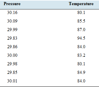
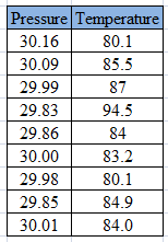
Hot enough for you? The following table presents the temperature, in degrees Fahrenheit, and barometric pressure, in inches of mercury, on August 15 at 12 noon in Macon. Georgia; over a nine-year period.
- Compute the least-squares regression line for predicting temperature from barometric pressure.
- Compute file coefficient of determination.
- Construct a
scatterplot of due temperature (y) versus the barometric pressure (x). - Which point is an outlier?
- Remove outlier and compute least-squares regression line for predicting temperature from barometric pressure.
- Is the outlier Explain.
- Compute the coefficient of determination for the data set with the outlier removed. Is the proportion of variation explained by the least-squares regression fine greater, less, or about the same without die outlier? Explain.
a.
The least squares regression line for the given data set.
Answer to Problem 23E
Explanation of Solution
Given information:
Belowtable represents the temperature, in degrees Fahrenheit, and barometric pressure, in inches of mercury, on August

Formula used:
The equation for least-square regression line:
Where
The correlation coefficient of a data is given by:
Where,
The standard deviations are given by:
Calculation:
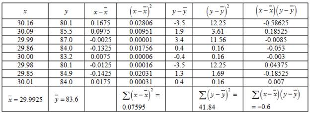
The mean of x is given by:
The mean of y is given by:
The data can be represented in tabular form as:
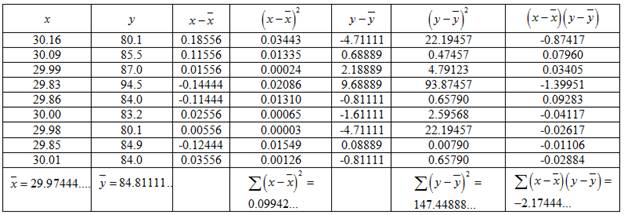
Hence, the standard deviation is given by:
And,
Consider,
Putting the values in the formula,
Putting the values to obtain
Putting the values to obtain
Hence, the least-square regression line is given by:
Therefore, the least squares regression line for the given data set is
b.
The coefficient of determination.
Answer to Problem 23E
Explanation of Solution
Given information:
Same as part
Calculation:
From part
The coefficient of determination is given by:
Where
Putting the values to obtain Coefficient of Determination,
Therefore, the Coefficient of Determination is
c.
Construct the scatterplot of the temperature
Explanation of Solution
Given information:
Below table represents the temperature, in degrees Fahrenheit, and barometric pressure, in inches of mercury, on August

Calculation:
The scatter plot can be drawn with the help of the given data. The Pressure will be taken on horizontal axis and the temperature will betaken on vertical axis.
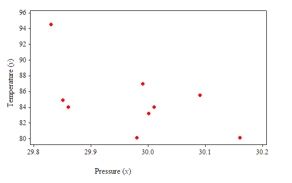
From the scatterplot, it is observed that there is a moderate association between the “variable temperature” and “barometric pressure”.
d.
The points which are outliers.
Answer to Problem 23E
Explanation of Solution
Given information:
Same as part
Calculation:
From above table, it can be seen that among all the
Therefore, the outlier point is
e.
The least squares regression line for the given data set excluding the outlier.
Answer to Problem 23E
Explanation of Solution
Given information:
Same as part
Formula used:
The equation for least-square regression line:
Where
The correlation coefficient of a data is given by:
Where,
The standard deviations are given by:
Calculation:
From part
Excluding the outlier,
The mean of
The mean of
The data can be represented in tabular form as:
Hence, the standard deviation is given by:
And,
Consider,
Putting the values in the formula,
Putting the values to obtain
Plugging the values to obtain
Hence, the least-square regression line is given by:
Therefore, the least squares regression line for the given data set by excluding the outlier is
f.
Whether the outlier is influential.
Answer to Problem 23E
The outlier is influential.
Explanation of Solution
Given information:
Same as part
Calculation:
From part
From part
From above equations, it can be observed that removing the outlier creates a great difference in the equation of the least square regression line.
Therefore, the outlier is influential.
g.
The coefficient of determination for the data set excluding the outliers.
Answer to Problem 23E
The proportion of variation is less without the outlier.
Explanation of Solution
Given information:
Same as part
Calculation:
The coefficient of determination is given by:
Where
From part
Putting the values to obtain Coefficient of Determination,
Therefore, the Coefficient of Determination is
Here the coefficient of determination reduced without the outlier.
Hence, the proportion of variance explained is less without the outlier.
Want to see more full solutions like this?
Chapter 4 Solutions
ELEM. STATISTICS TEXT W/ MANUAL+CONNECT


 College AlgebraAlgebraISBN:9781305115545Author:James Stewart, Lothar Redlin, Saleem WatsonPublisher:Cengage Learning
 Linear Algebra: A Modern IntroductionAlgebraISBN:9781285463247Author:David PoolePublisher:Cengage Learning
 Glencoe Algebra 1, Student Edition, 9780079039897...AlgebraISBN:9780079039897Author:CarterPublisher:McGraw Hill