UNDERSTANDING BASIC STAT LL BUND >A< F
7th Edition
ISBN: 9781337372763
Author: BRASE
Publisher: Cengage Learning
bartleby

Concept explainers

bartleby

Videos

Textbook Question
Book Icon
Chapter 4.2, Problem 11P

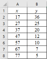
Auto Accidents: Age Data for this problem are based on information taken from The Wall Street Journal. Let x be the age in years of a licensed automobile driver. Let y be the percentage of all fatal accidents (for a given age) due to speeding. For example, the first data pair indicates that 36% of all fatal accidents involving 17-year-olds are due to speeding.

x 17 27 37 47 57 67 77
y 36 25 20 12 10 7 5

Complete parts (a) through (e), given x = 329 , y = 115 , x 2 = 18 , 263 , y 2 = 2639 , x y = 4015 , and r 0.959.

(f) Predict the percentage of all fatal accidents due to speeding for 25-year-olds.

(a)

Expert Solution
Check Mark
To determine

To graph: The scatter diagram for age in years of a licensed automobile driver (x) and percentage of all fatal accidents (y).

Explanation of Solution

Given: The data which consists of variables, ‘age of a licensed automobile driver (in years)’ and ‘the percentage of all fatal accidents (for a given age)’ due to speeding, represented by x and y respectively, is provided.

Graph:

Follow the steps given below in Excel to obtain the scatter diagram of the data.

Step 1: Enter the data into Excel sheet. The screenshot is given below.

UNDERSTANDING BASIC STAT LL BUND >A< F, Chapter 4.2, Problem 11P , additional homework tip  1

Step 2: Select the data and click on ‘Insert’. Go to charts and select the chart type ‘Scatter’.

UNDERSTANDING BASIC STAT LL BUND >A< F, Chapter 4.2, Problem 11P , additional homework tip  2

Step 3: Select the first plot and then click ‘add chart element’ provided in the left corner of the menu bar. Insert the ‘Axis titles’ and ‘Chart title’. The scatter plot for the provided data is shown below:

UNDERSTANDING BASIC STAT LL BUND >A< F, Chapter 4.2, Problem 11P , additional homework tip  3

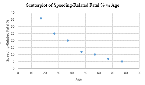
Interpretation: The scatterplot shows that, there is a negative correlation between the age of a licensed automobile drivers and the speeding- related fatal percentage. So, as the age increases, the fatal percentage related to speeding decreases and vice versa.

(b)

Expert Solution
Check Mark
To determine

To test: Whether the provided values of x, y, x2 ,y2, xy and r are correct or not.

Answer to Problem 11P

Solution: The provided values, that is, x=329, y=115, x2=18263, y2=2639 xy=4015 and r0.959 are correct.

Explanation of Solution

Given: The provided values are: x=329, y=115, x2=18263, y2=2639 xy=4015 and r0.959.

Calculation:

To compute x, y, x2 ,y2 and xy, it is easy to organize the data in a table of five columns and then add the values in each column. The table is given below:

x y x2 y2 xy
17 36 289 1296 612
27 25 729 625 675
37 20 1369 400 740
47 12 2209 144 564
57 10 3249 100 570
67 7 4489 49 469
77 5 5929 25 385
x=329 y=115 x2=18263 y2=2639 xy=4015

Now, the value of r can be calculated by using the formula below:

r=nxy-(x)(y)nx2(x)2ny2(y)2

Substituting the values in the above formula. Thus:

r=7(4015)(329)(115)(7)(18263)(329)2(7)(2639)(115)2=139144.89=0.959

Thus, the value of r0.959.

Conclusion: The provided values, x=329, y=115, x2=18263, y2=2639 xy=4015 and r0.959 have been verified.

(c)

Expert Solution
Check Mark
To determine

To find: The values of x¯,y¯, a, b and the equation for the least-squares line.

Answer to Problem 11P

Solution: The calculated values are, x¯=47 years,y¯=16.43%,a39.761 and b0.496. The least-squares line is,

y^=39.7610..496x.

Explanation of Solution

Given: The provided values are, x=329, y=115, x2=18263, y2=2639 xy=4015 and r0.959. The number of pairs of (x,y) in the data set (n) is 7.

Calculation:

The value of x¯ can be calculated as:

x¯=xn=3297=47

The value of y¯ can be calculated as:

y¯=yn=115716.43

The value of b can be calculated as:

b=nxy(x)(y)nx2(x)2=7(4015)(329)(115)7(18263)(329)2=9730196000.4964

The value of a can be calculated as:

a=y¯bx¯=16.43(0.4964×47)=16.43+23.330839.761

Therefore, the values are, x¯=47 years,y¯=16.43%,a39.761 and b0.496.

The general formula for the least-squares line is,

y^=a+bx

Here, a is the y-intercept and b is the slope.

Substitute the values of a and b in the general equation, to get the least-squares line of the data. That is,

y^=a+bx=39.761+(0.496)x=39.7610.496x

Therefore, the least-squares line is y^=39.7610.496x.

(d)

Expert Solution
Check Mark
To determine

To graph: The least-squares line on the scatter diagram which passes through the point (x¯,y¯).

Explanation of Solution

Given: The data which consists of variables, ‘age of a licensed automobile driver (in years)’ and ‘the fatal accidents percentage (for a given age) due to speeding’, represented by x and y respectively, is provided.

Graph:

Follow the steps given below in Excel to obtain the scatter diagram of the data.

Step 1: Enter the data into Excel sheet. The screenshot is given below.

UNDERSTANDING BASIC STAT LL BUND >A< F, Chapter 4.2, Problem 11P , additional homework tip  4

Step 2: Select the data and click on ‘Insert’. Go to charts and select the chart type ‘Scatter’.

UNDERSTANDING BASIC STAT LL BUND >A< F, Chapter 4.2, Problem 11P , additional homework tip  5

Step 3: Select the first plot and then click ‘add chart element’ provided in the left corner of the menu bar. Insert the ‘Axis titles’ and ‘Chart title’. The scatter plot for the provided data is shown below:

UNDERSTANDING BASIC STAT LL BUND >A< F, Chapter 4.2, Problem 11P , additional homework tip  6

Step 3: Right click on any data point and select ‘Add Trendline’. In the dialogue box, select ‘linear’ and check ‘Display Equation on Chart’

UNDERSTANDING BASIC STAT LL BUND >A< F, Chapter 4.2, Problem 11P , additional homework tip  7

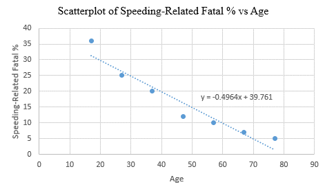
Interpretation: The least-squares line passes through the point (x¯,y¯)=(47,16.43) and the scatterplot displays the equation of the least-squares line as, y^=39.7610.4964x.

(e)

Expert Solution
Check Mark
To determine

The value of r2, the explained percentage of variation and the percentage of variation that is unexplained.

Answer to Problem 11P

Solution: The value of r2 is 0.920. The percentage of variation in fatal accident percentage due to speeding that can be explained by the age of the licensed automobile driver using the least-squares line is 92% and the rest 8% variation remains unexplained.

Explanation of Solution

Given: The value of the correlation coefficient (r) is 0.959.

Calculation: The coefficient of determination (r2) can be calculated as:

r2=(r)2=(0.959)20.920

Therefore, the value of r2 is 0.920.

The value of r2 indicates the proportion of total variation in y that can be explained by using the least-squares line. So, the explained percentage of variation in y is 92%.

Further, the proportion of variation in y that is unexplained can be calculated as:

1r2=10.920=0.08=8%

Hence, the percentage of variation in y that is unexplained is 8%.

Interpretation: About 92% of the variation in y (fatal % due to speeding) can be explained by the corresponding variation in x (age) and the least-squares line. The rest 8% of variation remains unexplained.

(f)

Expert Solution
Check Mark
To determine

To find: The predicted percentage of speeding related fatal accidents (y^) for 25-year-olds.

Answer to Problem 11P

Solution: The predicted value is approximately 27.36%.

Explanation of Solution

Given: The least-squares line from part (c) is, y^=39.7610.496x.

Calculation:

The predicted value (y^) for x=25 can be calculated as follows:

y^=39.7610.496x=39.7610.496(25)=39.76112.427.361

Thus, the value of y^27.36.

Interpretation: The percentage of all fatal accidents due to speeding for 25-years-olds is predicted to be 27.36%.

Want to see more full solutions like this?

Subscribe now to access step-by-step solutions to millions of textbook problems written by subject matter experts!

Chapter 4 Solutions

UNDERSTANDING BASIC STAT LL BUND >A< F

Ch. 4.1 - Interpretation Trevor conducted a study and found...Ch. 4.1 - Interpretation Do people who spend more time on...Ch. 4.1 - Veterinary Science: Shetland Ponies How much...Ch. 4.1 - Health Insurance:Administrative Cost The following...Ch. 4.1 - Meteorology: Cyclones Can a low barometer reading...Ch. 4.1 - Geology: Earthquakes Is the magnitude of an...Ch. 4.1 - Baseball: Batting Averages and Home Runs In...Ch. 4.1 - University Crime: FBI Report Do larger...Ch. 4.1 - Prob. 19PCh. 4.1 - Prob. 20PCh. 4.1 - Expand Your Knowledge: Using a Table to Test The...Ch. 4.1 - Expand Your Knowledge: Sample Size and...Ch. 4.1 - Prob. 23PCh. 4.2 - Statistical Literacy In the least-squares line...Ch. 4.2 - Statistical Literacy In the least squares line...Ch. 4.2 - Critical Thinking When we use a least-squares line...Ch. 4.2 - Critical Thinking If two variables have a negative...Ch. 4.2 - Critical Thinking: Interpreting Computer Printouts...Ch. 4.2 - Critical Thinking: Interpreting Computer Printouts...Ch. 4.2 - Economics: Entry-Level Jobs An economist is...Ch. 4.2 - Ranching: Cattle You are the foreman of the Bar-S...Ch. 4.2 - Weight of Car: Miles per Gallon Do heavier cars...Ch. 4.2 - Basketball: Fouls Data for this problem are based...Ch. 4.2 - Auto Accidents: Age Data for this problem are...Ch. 4.2 - Auto Accidents: Age Let x be the age of a licensed...Ch. 4.2 - Incoine: Medicai Care Let x be per capita income...Ch. 4.2 - Violent Crimes: Prisons Does prison really deter...Ch. 4.2 - Education: Violent Crime The following data are...Ch. 4.2 - Research: Patents The following data are based on...Ch. 4.2 - Archaeology: Artifacts Data for this problem are...Ch. 4.2 - Cricket Chirps: Temperature Anyone who has been...Ch. 4.2 - Expand Your Knowledge: Residual Plot The...Ch. 4.2 - Residual Plot: Miles per Gallon Consider the data...Ch. 4.2 - Expand Your knowledge: Logarithmic...Ch. 4.2 - Expand Your Knowledge: Logarithmic...Ch. 4.2 - Prob. 24PCh. 4.2 - Expand Your Knowledge: Logarithmic...Ch. 4 - Statistical Literacy Suppose the scatter diagram...Ch. 4 - Critical Thinking Suppose you and a friend each...Ch. 4 - Statistical Literacy When using the least-squares...Ch. 4 - StatisticalLiteracy Suppose that for x = 3. the...Ch. 4 - In Problems 9-14, (a) Draw a scatter diagram for...Ch. 4 - In Problems 9-14, (a) Draw a scatter diagram for...Ch. 4 - In Problems 9-14, (a) Draw a scatter diagram for...Ch. 4 - In Problems 9-14, (a) Draw a scatter diagram for...Ch. 4 - In Problems 9-14, (a) Draw a scatter diagram for...Ch. 4 - In Problems 9-14, (a) Draw a scatter diagram for...Ch. 4 - Prob. 1UTACh. 4 - Prob. 2UTACh. 4 - Prob. 3UTACh. 4 - Prob. 4UTACh. 4 - The data in this section are taken from this...Ch. 4 - The data in this section are taken from this...
Knowledge Booster
Background pattern image
Statistics
Learn more about
Need a deep-dive on the concept behind this application? Look no further. Learn more about this topic, statistics and related others by exploring similar questions and additional content below.
Recommended textbooks for you
Text book image
Linear Algebra: A Modern Introduction
Algebra
ISBN:9781285463247
Author:David Poole
Publisher:Cengage Learning
Text book image
Glencoe Algebra 1, Student Edition, 9780079039897...
Algebra
ISBN:9780079039897
Author:Carter
Publisher:McGraw Hill
Text book image
Functions and Change: A Modeling Approach to Coll...
Algebra
ISBN:9781337111348
Author:Bruce Crauder, Benny Evans, Alan Noell
Publisher:Cengage Learning
Text book image
Algebra & Trigonometry with Analytic Geometry
Algebra
ISBN:9781133382119
Author:Swokowski
Publisher:Cengage
Correlation Vs Regression: Difference Between them with definition & Comparison Chart; Author: Key Differences;https://www.youtube.com/watch?v=Ou2QGSJVd0U;License: Standard YouTube License, CC-BY
Correlation and Regression: Concepts with Illustrative examples; Author: LEARN & APPLY : Lean and Six Sigma;https://www.youtube.com/watch?v=xTpHD5WLuoA;License: Standard YouTube License, CC-BY