
Concept explainers
Videos
(a)
Section 1:
To find: The average and standard deviation of
(a)
Section 1:
Answer to Problem 23UYK
Solution: The sampling distribution
Explanation of Solution
Calculation: According to the central limit theorem, when a large sample n is selected from a population, with population average
Standard deviation of the sampling distribution
Section 2:
To find: The average and standard deviation of
Section 2:
Answer to Problem 23UYK
Solution: The sampling distribution
Explanation of Solution
Calculation: According to the central limit theorem, when a large sample n is selected from a population, with population average
Standard deviation of the sampling distribution
Section 3:
To find: The average and standard deviation of
Section 3:
Answer to Problem 23UYK
Solution: The sampling distribution
Explanation of Solution
Calculation: According to the central limit theorem, when a large sample n is selected from a population, with population average
Standard deviation of the sampling distribution
(b)
Section 1:
To find: The population distribution by using the Central Limit Theorem Applet.
(b)
Section 1:
Answer to Problem 23UYK
Solution: The distribution of the histogram has an average of 4.963 with standard deviation 2.019.
Explanation of Solution
Calculation: To obtain the population distribution by using the “Central Limit Theorem Applet,” follow the below steps:
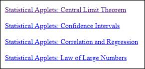
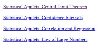
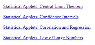
Step 1: Go to “Central Limit Theorem Applet” on the website. The screenshot is shown below:
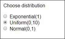
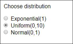
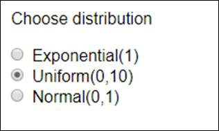
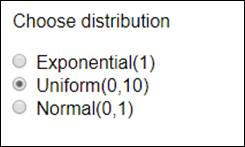
Step 2: Go to Choose distribution and select “Uniform(0,10).” The screenshot is shown below:
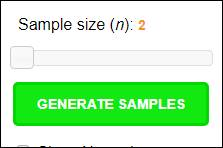
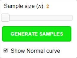
Step 3: Go to
The obtained result is shown below:
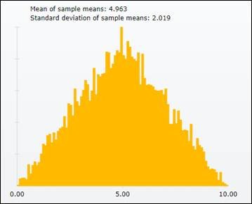
Interpretation: The distribution of the histogram has an average of 4.963 with standard deviation 2.019. All the values are near to the values that is calculated in part (a).
Section 2:
To find: The population distribution by using the Central Limit Theorem Applet.
Section 2:
Answer to Problem 23UYK
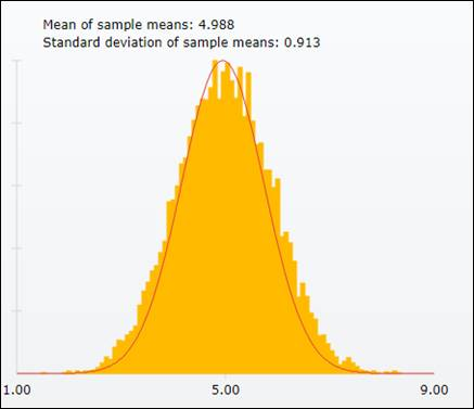
Solution: The distribution of the histogram has an average of 5.016 with standard deviation 0.915.
Explanation of Solution
Calculation: To obtain the population distribution by using the “Central Limit Theorem Applet,” follow the below steps:
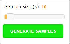
Step 1: Go to “Central Limit Theorem Applet” on the website. The screenshot is shown below:
Step 2: Go to Choose distribution and select “Uniform(0,10).” The screenshot is shown below:
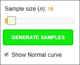
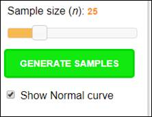
Step 3: Go to Sample size and specify n as “
The obtained result is shown below:
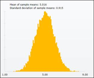
Interpretation: The distribution of the histogram has an average of 5.016 with standard deviation 0.915. All the values are near to the values that are calculated in part (a).
Section 3:
To find: The population distribution by using the Central Limit Theorem Applet.
Section 3:
Answer to Problem 23UYK
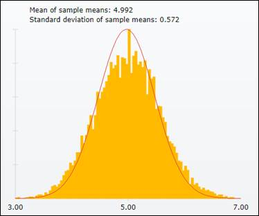
Solution: The distribution of the histogram has an average of 5.005 with standard deviation 0.575.
Explanation of Solution
Calculation: To obtain the population distribution by using the “Central Limit Theorem Applet,” follow the below steps:
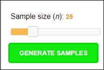
Step 1: Go to “Central Limit Theorem Applet” on the website. The screenshot is shown below:
Step 2: Go to Choose distribution and select “Uniform(0,10).” The screenshot is shown below:
Step3: Go to Sample size and specify n as “
The obtained result is shown below:
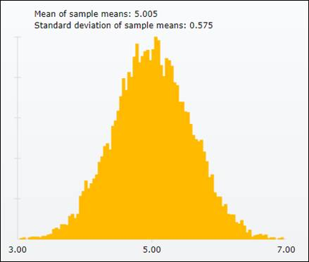
Interpretation: The distribution of the histogram has an average of 5.005 with standard deviation 0.575. All the values are near to the values that are calculated in part (a).
(c)
Section 1:
To find: The shape of the histogram and compare it with the normal plot.
(c)
Section 1:
Answer to Problem 23UYK
Solution: The shape of the distribution has bell-shaped curve. The shape of the histogram is close to the normal curve.
Explanation of Solution
Calculation: To compare the obtained histogram with the normal curve, follow the below steps:
Step 1: Go to “Central Limit Theorem Applet” on the website. The screenshot is shown below:
Step 2: Go to Choose distribution and select “Uniform(0,10).” The screenshot is shown below:
Step 3: Go to Sample size and specify n as “
The obtained result is shown below:
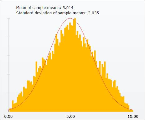
Interpretation: The obtained histogram is
Section 2:
To find: The shape of the histogram and compare it with the normal plot.
Section 2:
Answer to Problem 23UYK
Solution: The shape of the distribution has bell-shaped curve. The shape of the histogram is close to the normal curve.
Explanation of Solution
Calculation: To compare the obtained histogram with the normal curve, follow the steps below:
Step 1: Go to “Central Limit Theorem Applet” on the website. The screenshot is shown below:
Step 2: Go to Choose distribution and select “Uniform(0,10).” The screenshot is shown below:
Step 3: Go to Sample size and specify n as “
The obtained result is shown below:
Interpretation: The obtained histogram is normally distributed with bell-shaped curve. It can be concluded that the shape of the histogram is close to the normal curve.
Section 3:
To find: The shape of the histogram and compare it with the normal plot.
Section 3:
Answer to Problem 23UYK
Solution: The shape of the distribution is bell-shaped curve. The shape of the histogram is close to the normal curve.
Explanation of Solution
Calculation: To compare the obtained histogram with the normal curve, follow the below steps:
Step 1: Go to “Central Limit Theorem Applet” on the website. The screenshot is shown below:
Step 2: Go to Choose distribution and select “Uniform(0,10).” The screenshot is shown below:
Step 3: Go to Sample size and specify n as “
The obtained result is shown below:
Interpretation: The obtained histogram is normally distributed with bell-shaped curve. It can be concluded that the shape of the histogram is close to the normal curve.
(d)
The required sample size.
(d)
Answer to Problem 23UYK
Solution: The sample size should be 25.
Explanation of Solution
Want to see more full solutions like this?
Chapter 5 Solutions
Introduction to the Practice of Statistics


 MATLAB: An Introduction with ApplicationsStatisticsISBN:9781119256830Author:Amos GilatPublisher:John Wiley & Sons Inc
 Probability and Statistics for Engineering and th...StatisticsISBN:9781305251809Author:Jay L. DevorePublisher:Cengage Learning
 Statistics for The Behavioral Sciences (MindTap C...StatisticsISBN:9781305504912Author:Frederick J Gravetter, Larry B. WallnauPublisher:Cengage Learning
 Elementary Statistics: Picturing the World (7th E...StatisticsISBN:9780134683416Author:Ron Larson, Betsy FarberPublisher:PEARSON
 The Basic Practice of StatisticsStatisticsISBN:9781319042578Author:David S. Moore, William I. Notz, Michael A. FlignerPublisher:W. H. Freeman
 Introduction to the Practice of StatisticsStatisticsISBN:9781319013387Author:David S. Moore, George P. McCabe, Bruce A. CraigPublisher:W. H. Freeman