
Concept explainers
Videos
(a)
The values of n and p for X, which is binomially distributed.
(a)
Answer to Problem 69E
Solution: The required distribution of X is
Explanation of Solution
(b)
To find: The probability of every possible value of X.
(b)
Answer to Problem 69E
Solution: Probability distribution for each value of X is:
X |
|
0 |
0.02085 |
1 |
0.1360 |
2 |
0.333 |
3 |
0.3622 |
4 |
0.1477 |
Explanation of Solution
Calculation: In the provided problem the distribution can be calculated as:
For
For
For
For
For
Hence, the table representing every possible value of X and the probability parallel to X is shown below:
X |
|
0 |
0.02085 |
1 |
0.1360 |
2 |
0.333 |
3 |
0.3622 |
4 |
0.1477 |
To graph: A probability histogram for the obtained distribution.
Explanation of Solution
Graph: In the provided problem, the distribution of X is obtained in the part above. Now, the probability histogram can be obtained by using Minitab. The steps to be followed are enlisted below:
Step 1: Input the values of X and the probability in Minitab worksheet.
Step 2: Go to Graph > Histogram.
Step 3: Choose ‘View simple’ and click OK.
Step 4: Insert the value of X and the probability p in the column of graph variables.
Step 5: Click on Ok.
The Histogram is obtained as:
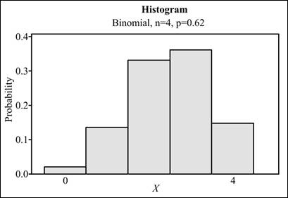
The probability histogram is obtained for the required distribution of X.
(c)
To Find: The average number of responders who said yes.
(c)
Answer to Problem 69E
Solution: The required average is 2.48.
Explanation of Solution
Calculation: Binomial
Substitute the values
The required average is 2.48.
To graph: The average value in the obtained histogram.
Explanation of Solution
Graph: The obtained average value is 2.48. To mark this value in the obtained histogram, the steps are as follows:
Step 1: Go to the histogram which is obtained above.
Step 2: Double click on the X axis.
Step 3: Select ‘Position of ticks’ and enter the obtained mean value 2.48.
Step 4: Click on Ok.
The histogram obtained is:
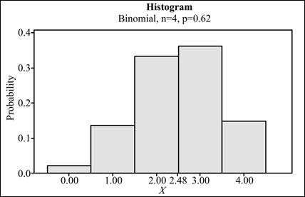
The histogram with the mark of mean value 2.48 is obtained.
Want to see more full solutions like this?
Chapter 5 Solutions
Introduction to the Practice of Statistics


 MATLAB: An Introduction with ApplicationsStatisticsISBN:9781119256830Author:Amos GilatPublisher:John Wiley & Sons Inc
 Probability and Statistics for Engineering and th...StatisticsISBN:9781305251809Author:Jay L. DevorePublisher:Cengage Learning
 Statistics for The Behavioral Sciences (MindTap C...StatisticsISBN:9781305504912Author:Frederick J Gravetter, Larry B. WallnauPublisher:Cengage Learning
 Elementary Statistics: Picturing the World (7th E...StatisticsISBN:9780134683416Author:Ron Larson, Betsy FarberPublisher:PEARSON
 The Basic Practice of StatisticsStatisticsISBN:9781319042578Author:David S. Moore, William I. Notz, Michael A. FlignerPublisher:W. H. Freeman
 Introduction to the Practice of StatisticsStatisticsISBN:9781319013387Author:David S. Moore, George P. McCabe, Bruce A. CraigPublisher:W. H. Freeman