Essentials of Business Analytics (MindTap Course List)
2nd Edition
ISBN: 9781305627734
Author: Jeffrey D. Camm, James J. Cochran, Michael J. Fry, Jeffrey W. Ohlmann, David R. Anderson
Publisher: Cengage Learning
expand_more
expand_more
format_list_bulleted
Concept explainers
Videos
Textbook Question
Chapter 8, Problem 21P
The president of a small manufacturing firm is concerned about the continual increase in manufacturing costs over the past several years. The following figures provide a time series of the cost per unit for the firm’s leading product over the past eight years:
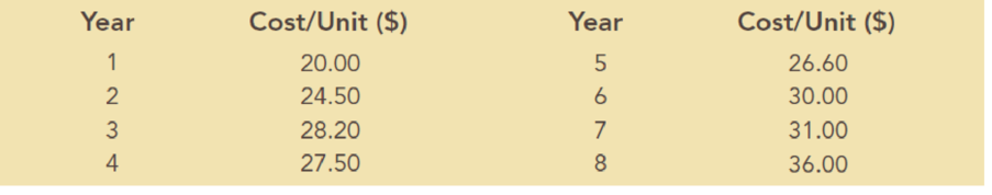
- a. Construct a time series plot. What type of pattern exists in the data?
- b. Use simple linear
regression analysis to find the parameters for the line that minimizes MSE for this time series. - c. What is the average cost increase that the firm has been realizing per year?
- d. Compute an estimate of the cost/unit for next year.
Expert Solution & Answer

Trending nowThis is a popular solution!

Students have asked these similar questions
The president of small manufacturing firm is concerned about the continual increase in manufacturing costs over the past several years. The following figures provide a time series of the cost per unit for the firm’s leading product over the past eight years.
Year
Cost/Unit ($)
Year
Cost/Unit ($)
1
20.00
5
26.60
2
24.50
6
30.00
3
28.20
7
31.00
4
27.50
8
36.00
Construct a time series plot. What type of pattern exists in the data?
Use simple linear regression analysis to find the parameters for the line that minimizes MSE for this time series.
What is the average cost increase that the firm has been realizing per year?
Compute an estimate of the cost/unit for next year.
A researcher notes that, in a certain region, a disproportionate number of software millionaires were born around the year 1955. Is this a coincidence, or does birth year matter when gauging whether a software founder will besuccessful? The researcher investigated this question by analyzing the data shown in the accompanying table. Complete parts a through c below.
a. Find the coefficient of determination for the simple linear regression model relating number (y) of software millionaire birthdays in a decade to total number (x) of births in the region. Interpret the result.
The coefficient of determination is 1.___?
(Round to three decimal places as needed.)
This value indicates that 2.____ of the sample variation in the number of software millionaire birthdays is explained by the
linear relationship with the total number of births in the region.
(Round to one decimal place as needed.)
b. Find the coefficient of determination for the simple linear regression model…
Consider the following estimated regression model relating annual salary to years of education and work experience.
Estimated Salary=10,737.30+2872.43(Education)+1129.1(Experience)Estimated Salary=10,737.30+2872.43(Education)+1129.1(Experience)
Suppose an employee with 44 years of education has been with the company for 1111 years (note that education years are the number of years after 8th8th grade). According to this model, what is his estimated annual salary?
Chapter 8 Solutions
Essentials of Business Analytics (MindTap Course List)
Ch. 8 - Consider the following time series data:
Using...Ch. 8 - Refer to the time series data in Problem 1. Using...Ch. 8 - Problems 1 and 2 used different forecasting...Ch. 8 - Consider the following time series data:
Compute...Ch. 8 - Consider the following time series...Ch. 8 - Consider the following time series...Ch. 8 - Refer to the gasoline sales time series data in...Ch. 8 - Prob. 8PCh. 8 - Prob. 9PCh. 8 - Prob. 10P
Ch. 8 - For the Hawkins Company, the monthly percentages...Ch. 8 - Corporate triple A bond interest rates for 12...Ch. 8 - The values of Alabama building contracts (in...Ch. 8 - The following time series shows the sales of a...Ch. 8 - Prob. 15PCh. 8 - The following table reports the percentage of...Ch. 8 - Consider the following time series: a. Construct a...Ch. 8 - Consider the following time series:
Construct a...Ch. 8 - Because of high tuition costs at state and private...Ch. 8 - The Seneca Children’s Fund (SCF) is a local...Ch. 8 - The president of a small manufacturing firm is...Ch. 8 - Consider the following time series: a. Construct a...Ch. 8 - Consider the following time series...Ch. 8 - The quarterly sales data (number of copies sold)...Ch. 8 - Prob. 25PCh. 8 - South Shore Construction builds permanent docks...Ch. 8 - Hogs & Dawgs is an ice cream parlor on the border...Ch. 8 - Donna Nickles manages a gasoline station on the...Ch. 8 - The Vintage Restaurant, on Captiva Island near...
Knowledge Booster


Learn more about
Need a deep-dive on the concept behind this application? Look no further. Learn more about this topic, statistics and related others by exploring similar questions and additional content below.Similar questions
- Consider the following estimated regression model relating annual salary to years of education and work experience. Estimated Salary=11,656.59+2985.74(Education)+1180.42(Experience)Estimated Salary=11,656.59+2985.74(Education)+1180.42(Experience) Suppose two employees at the company have been working there for five years. One has a bachelor's degree (88 years of education) and one has a master's degree (1010 years of education). How much more money would we expect the employee with a master's degree to makearrow_forwardFinally, the researcher considers using regression analysis to establish a linear relationship between the two variables – hours worked per week and yearly income. Hours per week Yearly Income ('000's) 18 43.8p 13 44.5 18 44.8 25.5 46.0 11.5 41.2 18 43.3 16 43.6 27 46.2 27.5 46.8 30.5 48.2 24.5 49.3 32.5 53.8 25 53.9 23.5 54.2 30.5 50.5 27.5 51.2 28 51.5 26 52.6 25.5 52.8 26.5 52.9 33 49.5 15 49.8 27.5 50.3 36 54.3 27 55.1 34.5 55.3 39 61.7 37 62.3 31.5 63.4 37 63.7 24.5 55.5 28 55.6 19 55.7 38.5 58.2 37.5 58.3 18.5 58.4 32 59.2 35 59.3 36 59.4 39 60.5 24.5 56.7 26 57.8 38 63.8 44.5 64.2 34.5 55.8 34.5 56.2 40 64.3 41.5 64.5 34.5 64.7 42.3 66.1 34.5 72.3 28 73.2 38…arrow_forwardFinally, the researcher considers using regression analysis to establish a linear relationship between the two variables – hours worked per week and yearly income. Hours per week Yearly Income ('000's) 18 43.8p 13 44.5 18 44.8 25.5 46.0 11.5 41.2 18 43.3 16 43.6 27 46.2 27.5 46.8 30.5 48.2 24.5 49.3 32.5 53.8 25 53.9 23.5 54.2 30.5 50.5 27.5 51.2 28 51.5 26 52.6 25.5 52.8 26.5 52.9 33 49.5 15 49.8 27.5 50.3 36 54.3 27 55.1 34.5 55.3 39 61.7 37 62.3 31.5 63.4 37 63.7 24.5 55.5 28 55.6 19 55.7 38.5 58.2 37.5 58.3 18.5 58.4 32 59.2 35 59.3 36 59.4 39 60.5 24.5 56.7 26 57.8 38 63.8 44.5 64.2 34.5 55.8 34.5 56.2 40 64.3 41.5 64.5 34.5 64.7 42.3 66.1 34.5 72.3 28 73.2 38…arrow_forward
- The following are data on the average weekly profits(in $1,000) of five restaurants, their seating capacities, andthe average daily traffic (in thousands of cars) that passestheir locations: Seating Traffic Weekly netcapacity count profitx1 x2 y120 19 23.8200 8 24.2150 12 22.0180 15 26.2240 16 33.5 (a) Assuming that the regression is linear, estimate β0, β1,and β2.(b) Use the results of part (a) to predict the averageweekly net profit of a restaurant with a seating capacityof 210 at a location where the daily traffic count averages14,000 cars.arrow_forwardThe following table shows the annual number of PhD graduates in a country in various fields. NaturalSciences Engineering SocialSciences Education 1990 70 10 70 30 1995 130 40 110 50 2000 330 130 280 140 2005 490 370 460 210 2010 590 550 830 520 2012 690 590 1,000 900 (a) With x = the number of social science doctorates and y = the number of education doctorates, use technology to obtain the regression equation. (Round coefficients to three significant digits.) y(x) = Graph the associated points and regression line. (b) What does the slope tell you about the relationship between the number of social science doctorates and the number of education doctorates? The slope tells us the increase in the number of social science doctorates for each additional education doctorate.The slope tells us the increase in the number of education doctorates for each additional social science doctorate. The slope tells us the decrease in the number…arrow_forwardThe following table shows the annual number of PhD graduates in a country in various fields. NaturalSciences Engineering SocialSciences Education 1990 70 10 60 30 1995 130 40 120 50 2000 330 130 280 140 2005 490 370 460 210 2010 590 550 830 520 2012 690 590 1,000 900 (a) With x = the number of social science doctorates and y = the number of education doctorates, use technology to obtain the regression equation. (Round coefficients to three significant digits.) y(x) = Graph the associated points and regression line. (b) What does the slope tell you about the relationship between the number of social science doctorates and the number of education doctorates? The slope tells us the increase in the number of education doctorates for each additional social science doctorate.The slope tells us the decrease in the number of education doctorates for each additional social science doctorate. The slope tells us the increase in the number…arrow_forward
- The operations manager of a musical instrument distributor feels that the demand for Bass Drums may be related to the number of television appearances by the popular rick group Green Shades during the previous month. The manager has collected the data shown in the following table. Demand for Bass Drums 3 6 7 5 10 8 Green Shades TV appearances 3 4 7 6 8 5 Develop the linear regression equation to forecast. Forecast demand for Bass Drums when Green Shades’ TV appearances are 10. Compute MSE and standard deviation for Problem 8.arrow_forwardSuppose a study wants to predict the market price of a certain species of turtle (Y) based on the following independent variables indicated in the table. Based from the table, what is the equation of the multiple linear regression? (Round off up to two decimal places. Market Price = 0.07 - 0.40*weight + 1.51*length + 1.41*width + 0.80*age Market Price = - 0.40*weight + 1.51*length + 1.41*width + 0.80*age Market Price = 0.07 + 0.40*weight + 1.51*length + 1.41*width + 0.80*age Market Price = 0.07 - 0.40 + weight + 1.51 + length + 1.41 + width + 0.80 + agearrow_forwardBased on the following data - (a) units produced from September to December are as follows: 18,900, 17,500, 21,200, 23,400; (b) total cost are as follows: P1,240,800, P1,198,000, P1,374,200, P1,563,800. What is the cost function using least-squares regression analysis?arrow_forward
- Compute the forecasted values for Yt for July and August in 2020 by using the modelsstated in (c) and (d)arrow_forwardConsider the following time series: Quarter Year 1 Year 2 Year 3 1 66 63 57 2 48 40 50 3 59 61 54 4 73 76 67 (a) Choose a time series plot. (i) (ii) (iii) (iv) What type of pattern exists in the data? Is there an indication of a seasonal pattern? (b) Use a multiple linear regression model with dummy variables as follows to develop an equation to account for seasonal effects in the data: Qtr1 = 1 if quarter 1, 0 otherwise; Qtr2 = 1 if quarter 2, 0 otherwise; Qtr3 = 1 if quarter 3, 0 otherwise. For subtractive or negative numbers use a minus sign even if there is a + sign before the blank (Example: -300). ŷ = ?? + ?? Qtr1 +?? Qtr2 + ?? Qtr3 (c) Compute the quarterly forecasts for next year. Year Quarter Ft 4 1 4 2 4 3 4 4arrow_forwardCascade Pharmaceuticals Company developed the following regression model, using time-series data from the past 33 quarters, for one of its nonprescription cold remedies: Y=−1.04+0.24X1−0.27X2�=−1.04+0.24�1−0.27�2 where Y� = quarterly sales (in thousands of cases) of the cold remedy X1�1 = Cascade's quarterly advertising (× $1,000) for the cold remedy X2�2 = competitors' advertising for similar products (× $10,000) Here is additional information concerning the regression model: sb1=0.042�b1=0.042, sb2=0.070�b2=0.070, R2=0.720�2=0.720, se=1.63��=1.63, F-statistic=31.402F-statistic=31.402, and Durbin-Watson (d) statistic=0.499Durbin-Watson (d) statistic=0.499. Which of the independent variables (if any) appears to be statistically significant (at the 0.05 level) in explaining sales of the cold remedy? (Hint: t0.05/2,33 - 3=2.042�0.05/2,33 - 3=2.042.) Check all that apply. X1�1 X2�2 What proportion of the total variation in sales is explained by the regression…arrow_forward
arrow_back_ios
SEE MORE QUESTIONS
arrow_forward_ios
Recommended textbooks for you
 College AlgebraAlgebraISBN:9781305115545Author:James Stewart, Lothar Redlin, Saleem WatsonPublisher:Cengage Learning
 Linear Algebra: A Modern IntroductionAlgebraISBN:9781285463247Author:David PoolePublisher:Cengage Learning
College Algebra
Algebra
ISBN:9781305115545
Author:James Stewart, Lothar Redlin, Saleem Watson
Publisher:Cengage Learning
Linear Algebra: A Modern Introduction
Algebra
ISBN:9781285463247
Author:David Poole
Publisher:Cengage Learning
Correlation Vs Regression: Difference Between them with definition & Comparison Chart; Author: Key Differences;https://www.youtube.com/watch?v=Ou2QGSJVd0U;License: Standard YouTube License, CC-BY
Correlation and Regression: Concepts with Illustrative examples; Author: LEARN & APPLY : Lean and Six Sigma;https://www.youtube.com/watch?v=xTpHD5WLuoA;License: Standard YouTube License, CC-BY