Videos
Interpretation:
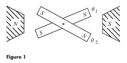
For a bar magnet system
Concept Introduction:
Determine the fixed point for the given system.
Determine the bifurcation using the Jacobian matrix and fixed point.
Sketch phase portrait using system equation.
Answer to Problem 12E
Solution:
The fixed point of the system is
It is shown that a bifurcation occurs at
It is shown that the system is a “gradient” system,
It is proved that the system has no periodic orbits.
The phase portrait for
Explanation of Solution
Consider the Interacting bar magnets system with system equation
To calculate the fixed point of the system, equationsare as:
For the calculation of the fixed point of the above system equation, first equating the first derivative of the above system equation to zero.
Substitute
From the trigonometric identity,
Hence,
Substitute
From the trigonometric identity,
To obtain
Using trigonometric identity,
Apply trigonometric expression in the above expression of the fixed point,
From the above,
By solving,
Similarly,
Compare the above expression of
Substitute
Therefore, the fixed point of the above system equation is
Bifurcation is defined as the point or area at which something is divided into two parts and branches. The point in the system equation at which bifurcating occur.
For the calculation of the type of bifurcation, the Jacobian matrix is:
By substituting
The Jacobian matrix at the fixed point
The trace of the above Jacobian matrix is calculated as:
The determinant of the above Jacobian matrix is calculated as:
Therefore, from the above calculation of the system equation, the determinant of the above system equation at the fixed point is zero, so the bifurcation is saddle node bifurcation.
The calculation of the potential gradient of the given systemis shown below.
The expression of the potential function is:
Substitute
Therefore, the potential function for the value of
Similarly, for
Substitute
Therefore, the potential function for the value of
For the calculation of the periodic orbit,
Add the potential function.
From the trigonometric identity,
Hence,
For the periodicity of the above system equation, calculate the closed orbit of the above system equation with the help of the Greens theorem,
Therefore, from above calculation of the potential function, it is clear that the system has no periodic orbit.
A phase portrait is defined as the geometrical representation of the trajectories of the dynamical system in the phase plane of the system equation. Every set of the initial condition is represented by a different curve or point in the phase plane.
The phase portrait for the given system equation is shown. The system equations are given as:
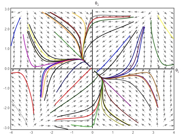
The phase portrait plot for the above system equation for the value of K lying in the range of
The phase portrait of the above system equation at
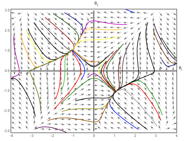
The phase portrait plot for the above system equation for the value of K lying in the range of
The phase portrait of the above system equation at
Want to see more full solutions like this?
Chapter 8 Solutions
Nonlinear Dynamics and Chaos


 Advanced Engineering MathematicsAdvanced MathISBN:9780470458365Author:Erwin KreyszigPublisher:Wiley, John & Sons, Incorporated
 Numerical Methods for EngineersAdvanced MathISBN:9780073397924Author:Steven C. Chapra Dr., Raymond P. CanalePublisher:McGraw-Hill Education
 Introductory Mathematics for Engineering Applicat...Advanced MathISBN:9781118141809Author:Nathan KlingbeilPublisher:WILEY
 Mathematics For Machine TechnologyAdvanced MathISBN:9781337798310Author:Peterson, John.Publisher:Cengage Learning,
