
Videos
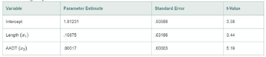
Highway crash data analysis. Researchers at Montana State University have written a tutorial on an empirical method for analyzing before and after highway crash data (Montana Department of Transportation, Research Report, May 2004). The initial step in the methodology is to develop a Safety Performance
Interstate Highways
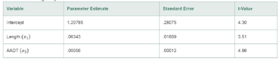
Noninterstate Highways
- a. Give the least squares prediction equation for the interstate highway model.
- b. Give practical interpretations of the β estimates, part a.
- c. Refer to part a. Find a 99% confidence interval for β1 and interpret the result.
- d. Refer to part a. Find a 99% confidence interval for β2 and interpret the result.
- e. Repeat parts a-d for the noninterstate highway model.
- f. Write a first-order model for E(y) as a function of x1 and x2 that allows the slopes to differ depending on whether the roadway segment is Interstate or non-interstate. [Hint: Create a dummy variable for Interstate/non-interstate.]
Want to see the full answer?
Check out a sample textbook solution
Chapter 12 Solutions
Statistics For Business And Economics Plus Mystatlab With Pearson Etext -- Access Card Package (13th Edition)


- The accompanying data file contains 40 observations on the response variable y along with the predictor variables x and d. Consider two linear regression models where Model 1 uses the variables x and d and Model 2 extends the model by including the interaction variable xd. Use the holdout method to compare the predictability of the models using the first 30 observations for training and the remaining 10 observations for validation. y x d 70 11 1 102 19 1 76 12 1 83 14 1 61 17 0 62 13 0 67 20 0 98 16 1 84 11 1 101 15 1 51 16 0 108 16 1 32 13 0 71 15 1 101 17 1 90 15 1 112 19 1 88 13 1 110 18 1 95 17 1 44 14 0 51 19 0 112 17 1 113 17 1 52 13 0 61 10 1 100 16 1 78 14 1 90 16 1 57 16 0 59 15 0 53 15 0 119 19 1 109 18 1 68 11 0 104 19 1 45 18 0 67 17 0 65 15 0 74 14 1 1. Use the training set to estimate Models 1 and 2. Note: Negative values should be indicated by a minus sign. Round your answers to 2…arrow_forwardIn a typical multiple linear regression model where x1 and x2 are non-random regressors, the expected value of the response variable y given x1 and x2 is denoted by E(y | 2,, X2). Build a multiple linear regression model for E (y | *,, *2) such that the value of E(y | x1, X2) may change as the value of x2 changes but the change in the value of E(y | X1, X2) may differ in the value of x1 . How can such a potential difference be tested and estimated statistically?arrow_forwardFor the regression model Yi = b0 + eI, derive the least squares estimator.arrow_forward
- In a laboratory experiment, data were gathered on the life span (y in months) of 33 rats, units of daily protein intake (x1), and whether or not agent x2 (a proposed life-extending agent) was added to the rats' diet (x2 = 0 if agent x2 was not added, and x2 = 1 if agent was added). From the results of the experiment, the following regression model was developed:ŷ = 36 + .8x1 − 1.7x2Also provided are SSR = 60 and SST = 180.The test statistic for testing the significance of the model is _____. a. 5.00 b. .50 c. .25 d. .33arrow_forwardDoes correcting the sugar cane model for heteroscedasticity improve its performance? Interpret the regression coefficients.arrow_forwardgive handwritten answer of the question-Which one of the following is the most used model or calibration curve for a one-component system in quantitative analysis? Y = bo + b1X1 + b2X2 + error Y = bo + b1X + b1X2 + error Y = bo + b1X + error Y = bo + b1X1 + b2X2 + b3X1X2 + errorarrow_forward
- The accompanying data file contains 40 observations on the response variable y along with the predictor variables x1 and x2. Use the holdout method to compare the predictability of the linear model with the exponential model using the first 30 observations for training and the remaining 10 observations for validation. y x1 x2 533.86 20 30 104.84 15 20 64.89 20 23 159.61 16 21 43.06 13 16 4.27 13 13 736.56 15 30 64.89 20 23 10.64 20 22 76.90 18 20 4.89 11 13 80.90 11 16 224.17 12 19 45.75 16 25 8.13 17 17 319.97 13 30 48.61 19 25 564.67 12 27 111.87 11 25 152.39 13 24 13.34 18 14 28.80 15 22 37.56 13 15 105.62 17 26 44.05 18 21 451.65 17 28 10.34 18 21 32.70 12 13 19.21 14 12 14.02 15 16 2.45 16 12 2.48 20 15 50.34 17 21 29.31 17 20 33.75 16 12 196.28 17 29 943.12 13 30 7.25 10 12 89.73 15 25 32.91 12 18 1. Use the training set to estimate Models 1 and 2. Note: Negative values should be indicated by a…arrow_forwardAfter we have conducted a hypothesis test, what are two ways we could measure the effect size of the hypothesized relationship? Be sure to provide the equations and a description of what they tell usarrow_forwardThe table shows a part of an output of a linear regression model predicting the average fare on different flight routes. Data Table Regression Table Coefficient Constant 95.80976147 COUPON −9.61654124 DISTANCE 0.080733811 PAX −0.000167343 What is the difference in prediction of the following two routes? Route A that is 3,000 miles, with COUPON=1.5 and PAX=6,000 Route B that is 3,000 miles, with COUPON=1.2 and PAX=6,000.arrow_forward
- Data was collected on 54 observations on a response of interest, y, and four potential predictor variables x1, x2, x3, and x4. The output from regression analyses of the data is attached to the end of the page. d) Is the variable from your best simple linear regression model (from part a) included in the model with the lowest overall MSE (part b)? Briefly explain why it could happen that the best single variable is not in the best overall model. e) Following the best subsets regression results, the sums of squares for regression and error (also called residual) are displayed for several models. Using the regression sums of squares information for the full model containing all four x variables, calculate i) the R2 value for the full model, ii) the F statistic for the test of the H0: b1 = b2 = b3 = b4 = 0, and iii) the standard deviation of the residuals for the full model. f) Using the regression sums of squares information, test the null hypothesis H0:b2 = b4 = 0 for the full model.…arrow_forwardDoes the sugar cane model suffer from heteroscedasticity? Perform a Breusch-Pegan test as well as a Whitetest to verify what the residual plots suggests, based on the following regression results:arrow_forwardA fitted linear regression model is (y=10+2x ). If x = 0 and the corresponding observed value of y = 9, the residual at this observation is:arrow_forward
 MATLAB: An Introduction with ApplicationsStatisticsISBN:9781119256830Author:Amos GilatPublisher:John Wiley & Sons Inc
 Probability and Statistics for Engineering and th...StatisticsISBN:9781305251809Author:Jay L. DevorePublisher:Cengage Learning
 Statistics for The Behavioral Sciences (MindTap C...StatisticsISBN:9781305504912Author:Frederick J Gravetter, Larry B. WallnauPublisher:Cengage Learning
 Elementary Statistics: Picturing the World (7th E...StatisticsISBN:9780134683416Author:Ron Larson, Betsy FarberPublisher:PEARSON
 The Basic Practice of StatisticsStatisticsISBN:9781319042578Author:David S. Moore, William I. Notz, Michael A. FlignerPublisher:W. H. Freeman
 Introduction to the Practice of StatisticsStatisticsISBN:9781319013387Author:David S. Moore, George P. McCabe, Bruce A. CraigPublisher:W. H. Freeman