
Concept explainers
Videos
The article “Performance Test Conducted for a Gas Air-Conditioning System” (American Society of Heating, Refrigerating, and Air Conditioning Engineering [1969]: 54) reported the following data on maximum outdoor temperature (x) and hours of chiller operation per day (y) for a 3-ton residential gas air-conditioning system:
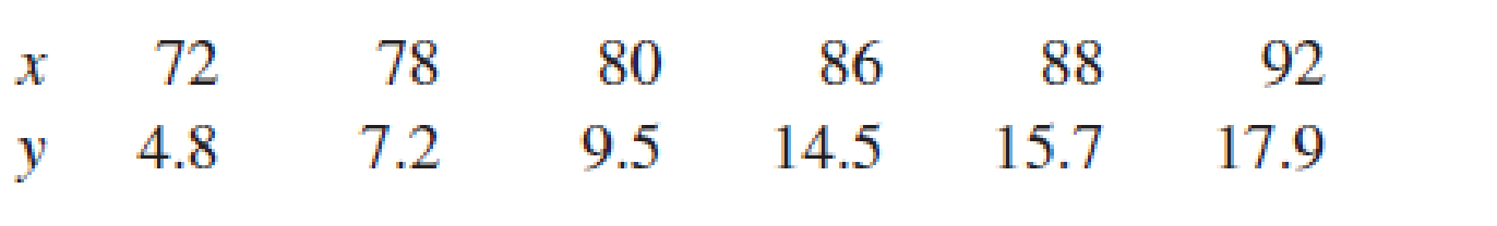
Suppose that the system is actually a prototype model, and the manufacturer does not wish to produce this model unless the data strongly indicate that when maximum outdoor temperature is 82°F. The true average number of hours of chiller operation is less than 12. The appropriate hypotheses are then
H0: α + β(82) = 12 versus Ha: α + β(82) < 12
Use the statistic
which has a t distribution based on (n – 2) df when H0 is true, to test the hypotheses at significance level 0.01.
Want to see the full answer?
Check out a sample textbook solution
Chapter 13 Solutions
INTRODUCTION TO STATISTICS & DATA ANALYS


- Consider the following two a.m. peak work trip generation models, estimated by household linear regression: T = 0.62 + 3.1 X1 + 1.4 X2 R2= 0.590 (2.3) (7.1) (5.9) T = 0.01 + 2.4 X1 + 1.2 Z1 + 4.0 Z2 R2= 0.598 (0.8) (4.2) (1.7) (3.1) X1 = number of workers in the household X2 = number of cars in the household, Z1 is a dummy variable which takes the value 1 if the household has one car, Z2 is a dummy variable which takes the value 1 if the household has two or more cars. Compare the two models and choose the best. If a zone has 1000 households, of which 50% have no car, 35% have one car, and the rest have exactly two cars, estimate the total number of trips generated by this zone. Use the preferred trip generation model and assume that each household has an average of two workersarrow_forwardThe article “Withdrawal Strength of Threaded Nails” (D. Rammer, S. Winistorfer, and D. Bender, Journal of Structural Engineering 2001:442–449) describes an experiment comparing the ultimate withdrawal strengths (in N/mm) for several types of nails. For an annularly threaded nail with shank diameter 3.76 mm driven into spruce-pine-fir lumber, the ultimate withdrawal strength was modeled as lognormal with μ = 3.82 and σ = 0.219. For a helically threaded nail under the same conditions, the strength was modeled as lognormal with μ = 3.47 and σ = 0.272. a) What is the mean withdrawal strength for annularly threaded nails? b) What is the mean withdrawal strength for helically threaded nails? c) For which type of nail is it more probable that the withdrawal strength will be greater than 50 N/mm? d) What is the probability that a helically threaded nail will have a greater withdrawal strength than the median for annularly threaded nails? e) An experiment is performed in which withdrawal…arrow_forwardFor b there are two cases and for c I have to plug the initial data into the odearrow_forward
- A consumer buying cooperative tested the effective heating area of 20 different electric space heaters with different wattages. Here are the results. Heater Wattage Area 1 1,000 290 2 750 292 3 1,500 148 4 1,250 246 5 1,250 203 6 750 85 7 1,250 237 8 1,000 139 9 1,500 64 10 1,000 171 11 1,750 163 12 1,250 175 13 750 264 14 1,500 50 15 1,750 163 16 1,500 177 17 1,250 118 18 1,750 122 19 1,000 144 20 1,500 103 Click here for the Excel Data File Compute the correlation between the wattage and heating area. Is there a direct or an indirect relationship? (Round your answer to 4 decimal places.) Conduct a test of hypothesis to determine if it is reasonable that the coefficient is greater than zero. Use the 0.025 significance level. (Round intermediate calculations and final answer to 3 decimal places.) H0: ρ ≤ 0; H1: ρ > 0 Reject H0 if t…arrow_forwardRefer to Exercise 8.S.6. Analyze these data using a Wilcoxon signed-rank test.arrow_forwardIn a typical multiple linear regression model where x1 and x2 are non-random regressors, the expected value of the response variable y given x1 and x2 is denoted by E(y | 2,, X2). Build a multiple linear regression model for E (y | *,, *2) such that the value of E(y | x1, X2) may change as the value of x2 changes but the change in the value of E(y | X1, X2) may differ in the value of x1 . How can such a potential difference be tested and estimated statistically?arrow_forward
- A consumer buying cooperative tested the effective heating area of 20 different electric space heaters with different wattages. Here are the results. Heater Wattage Area 1 1,000 108 2 750 291 3 1,500 100 4 1,000 43 5 1,250 68 6 1,500 181 7 1,250 254 8 750 228 9 1,500 126 10 1,500 166 11 750 45 12 750 237 13 1,000 75 14 1,750 126 15 1,750 249 16 1,750 105 17 1,750 298 18 1,250 212 19 750 98 20 750 185 Click here for the Excel Data File a. Compute the correlation between the wattage and heating area. Is there a direct or an indirect relationship? (Round your answer to 4 decimal places.) b. Conduct a test of hypothesis to determine if it is reasonable that the coefficient is greater than zero. Use the 0.050 significance level. (Round intermediate calculations and final answer to 3 decimal places.)H0: ρ ≤ 0; H1: ρ > 0 Reject H0 if t > 1.734…arrow_forwardConsider the following regression model Yt = β0 + β1 Ut + β2 Vt + β3 Wt + β4Xt + ∈t , where U, V, W, X and Y are economic variables observed from t = 1, . . . , 75, β0 , . . . , β4 are the model parameters and ∈t is the random disturbance term satisfying the classical assumptions. Ordinary Least Squares (OLS) is used to estimate the parameters, producing the following estimated model: Yt = 1.115 + 0.790*Ut − 0.327*Vt + 0.763*Wt + 0.456*Xt (0.405) (0.178) (0.088) (0.274) (0.017) where standard errors are given in parentheses, the R-squared = 0.941, the Durbin-Watson statistic is DW = 1.907 and the residual sum of squares is RSS = 0.0757. In answering this question, use the 5% level of significance for any hypothesis tests that you are asked to perform, state clearly the null and al- ternative hypotheses that you are testing, the test statistics that you are using and interpret the decisions that you make.…arrow_forwardCompute the forecasted values for Yt for July and August in 2020 by using the modelsstated in (c) and (d)arrow_forward
- f X1,X2,...,Xn constitute a random sample of size n from a geometric population, show that Y = X1 + X2 + ···+ Xn is a sufficient estimator of the parameter θ.arrow_forwardSuppose that Yt follows a stationary AR(1) model with β0 = 0 and β1 = 0.5.If Yt = 10, what is your forecast of Yt+2 (that is, what is Yt+2|t)? What isYt+h|t for h = 20? Does this forecast for h = 20 seem reasonable to you?arrow_forwardThe following Minitab display gives information regarding the relationship between the body weight of a child (in kilograms) and the metabolic rate of the child (in 100 kcal/ 24 hr). Predictor Coef SE Coef T PConstant 0.8570 0.4148 2.06 0.84Weight 0.38243 0.02978 13.52 0.000 S = 0.517508 R-Sq = 97.4% (a) Write out the least-squares equation. y^= ______ + _____x (b) For each 1 kilogram increase in weight, how much does the metabolic rate of a child increase? (Use 5 decimal places.)arrow_forward
 MATLAB: An Introduction with ApplicationsStatisticsISBN:9781119256830Author:Amos GilatPublisher:John Wiley & Sons Inc
 Probability and Statistics for Engineering and th...StatisticsISBN:9781305251809Author:Jay L. DevorePublisher:Cengage Learning
 Statistics for The Behavioral Sciences (MindTap C...StatisticsISBN:9781305504912Author:Frederick J Gravetter, Larry B. WallnauPublisher:Cengage Learning
 Elementary Statistics: Picturing the World (7th E...StatisticsISBN:9780134683416Author:Ron Larson, Betsy FarberPublisher:PEARSON
 The Basic Practice of StatisticsStatisticsISBN:9781319042578Author:David S. Moore, William I. Notz, Michael A. FlignerPublisher:W. H. Freeman
 Introduction to the Practice of StatisticsStatisticsISBN:9781319013387Author:David S. Moore, George P. McCabe, Bruce A. CraigPublisher:W. H. Freeman