
Videos
a.
Check whether the data contradict the prior belief.
State and test the appropriate hypotheses using a 0.10 level of significance.
a.
Explanation of Solution
The data is on age (x) and percentage of cribriform area of the lamina scleralis occupied by pores (y). The researchers believed that the average decrease in percentage area associated with a 1 year age increase was 0.5%.
1.
Here,
2.
Null hypothesis:
That is, the average decrease in percentage area is 0.5.
3.
Alternative hypothesis:
That is, the average decrease in percentage area is not 0.5.
4.
Here, the significance level is
5.
Test Statistic:
The formula for test statistic is,
In the formula, b denotes the estimated slope,
6.
The data are plotted in the scatter plot below.
If the scatterplot of the data shows a linear pattern, and the vertical variability of points does not appear to be changing over the range of x values in the sample, then it can be said that the data is consistent with the use of the simple linear regression model.
Software procedure:
Step-by-step procedure to obtain the scatterplot using MINITAB software:
- Choose Graph>Scatter plot.
- Select Simple.
- Click OK.
- Under Y variables, enter the column of y.
- Under X variables, enter the column of x.
- Click OK.
The output using MINITAB software is given below:
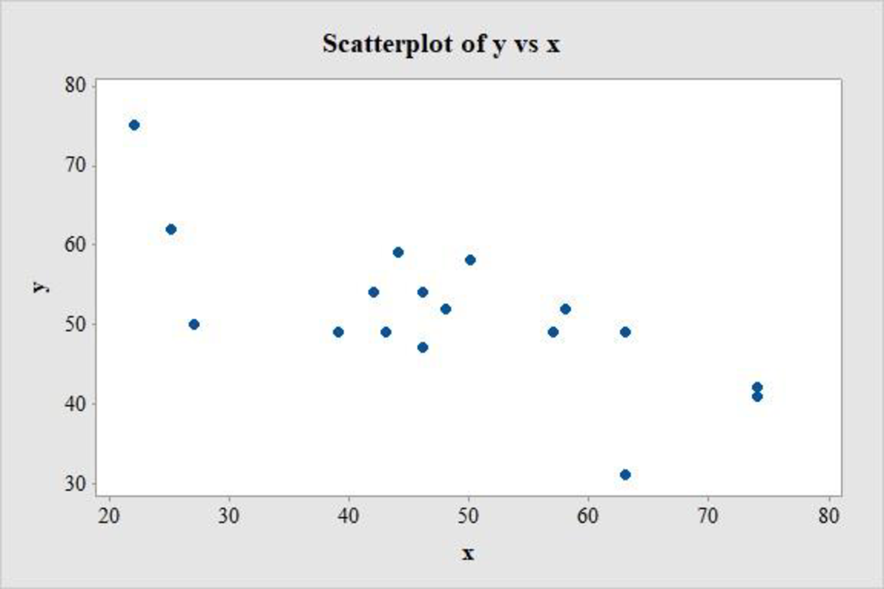
The scatter plot shows no apparent curve and there are no extreme observations. There is no change in the y values as the value of x changes and there are no influential points. Therefore, the simple linear regression model seems appropriate for the data set.
Assumption:
Here, the assumption made is that, the simple linear regression model is appropriate.
7.
Calculation:
The values required for the calculation of t is obtained in the following steps:
Software procedure:
Step-by-step procedure to obtain regression line using MINITAB software:
- Choose Stat > Regression > Regression > Fit Regression Model.
- Under Responses, enter the column of values y.
- Under Continuous predictors, enter the column of values x.
- Click OK.
Output using MINITAB software is given below:
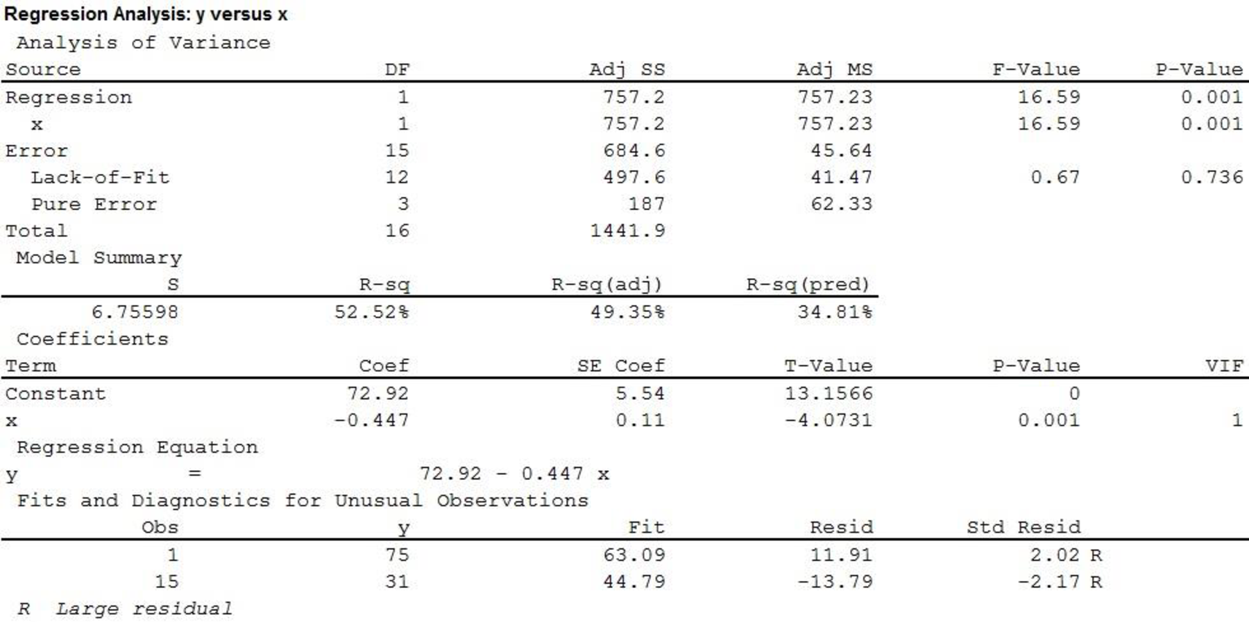
Since, the output provides test statistic value for a hypothesized mean of 0, the test statistic value for a hypothesized mean of –0.5 is obtained below.
For the given x values,
Substitute,
Hence, the test statistic value is 0.488.
8.
Formula for Degrees of freedom:
The formula for degrees of freedom is as follows:
Degrees of freedom:
The number of data values given are 17, that is
P-value:
Formula for p-value:
The P-value is,
The test statistic value is 0.488. The value of
Software procedure:
Step-by-Step procedure to find probability using MINITAB software:
- Choose Graph > Probability Distribution Plot.
- Choose View Probability > OK.
- From Distribution, choose ‘t’ distribution.
- Enter Degrees of freedom as 15.
- Click the Shaded Area tab.
- Choose X Value and Right tail for the region of the curve to shade.
- Enter the X value as 0.488.
- Click OK.
Output using MINITAB software is as follows:
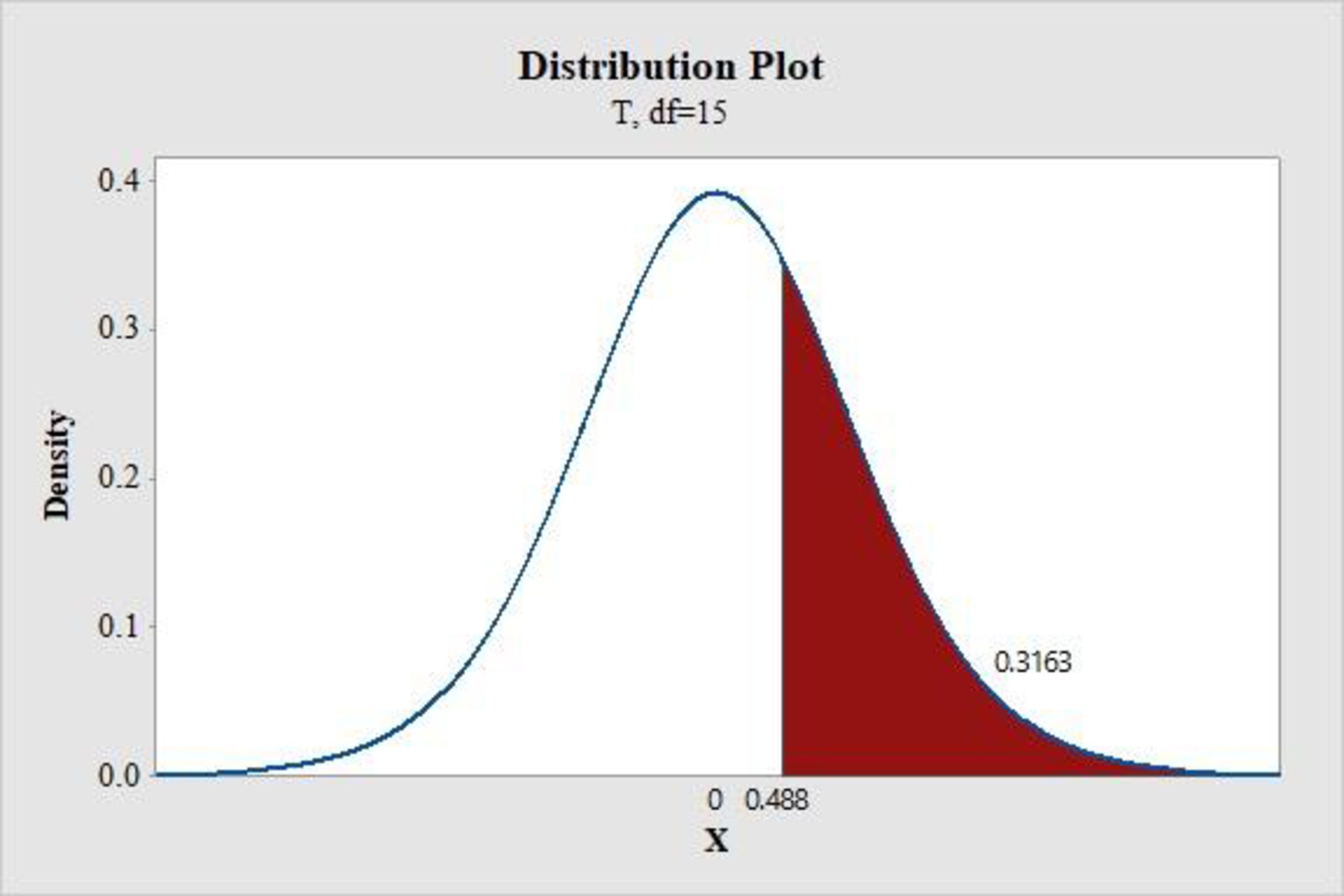
Thus,
P-value:
Thus, the p-value is 0.633.
9.
Rejection rule:
If
Conclusion:
The P-value is 0.633.
The level of significance is 0.1.
The P-value is greater than the level of significance.
That is,
Based on rejection rule, do not reject the null hypothesis.
Thus, there is no convincing evidence that the average decrease in percentage area associated with a 1-year age increase is not 0.5.
b.
Obtain an estimate of the average percentage area covered by pores for all 50-year olds in the population.
b.
Answer to Problem 61CR
The estimate of the average percentage area covered by pores for all 50-year olds in the population is between 47.05 and 54.08.
Explanation of Solution
Calculation:
The confidence interval for
From the MINITAB output in Part (a), the estimated linear regression line is
Point estimate:
The point estimate when the percentage area covered by pores for all 50-year olds in the population is calculated as follows.
Estimated standard deviation:
Substitute,
Critical value:
From the Appendix: Table 3 the t Critical Values:
- Locate the value 15 in the degrees of freedom (df) column.
- Locate the 0.95 in the row of central area captured.
- The intersecting value that corresponds to the df 15 with confidence level 0.95 is 2.13.
Thus, the critical value for
Substitute
Therefore, one can be 95% confident that the estimate of the average percentage area covered by pores for all 50-year olds in the population is between 47.05 and 54.08.
Want to see more full solutions like this?
Chapter 13 Solutions
INTRODUCTION TO STATISTICS & DATA ANALYS


- Low-Birth-Weight Hospital Stays. Data on low-birthweight babies were collected over a 2-year period by 14 participating centers of the National Institute of Child Health and Human Development Neonatal Research Network. Results were reported by J. Lemons et al. in the on-line paper “Very Low Birth Weight Outcomes of the National Institute of ChildHealth and Human Development Neonatal Research Network” (Pediatrics, Vol. 107, No. 1, p. e1). For the 1084 surviving babies whose birth weights were 751– 1000 grams, the average length of stay in the hospital was 86 days, although one center had an average of 66 days and another had an average of 108 days. a. Can the mean lengths of stay be considered population means? Explain your answer.b. Assuming that the population standard deviation is 12 days, determine the z-score for a baby’s length of stay of 86 days at the center where the mean was 66 days.c. Assuming that the population standard deviation is 12 days, determine the z-score for a…arrow_forwardWhen investigating the relationship between aerobic exercise capacity (as measured by VO2max, a continuous variable) and serum concentration of vitamin D, the authors of this study report a Pearson correlation coefficient estimate of r = 0.23 with a p-value of <0.01. Interpret.arrow_forwardAn experiment was conducted to compare the alcohol content of soy sauce on two different production lines. Production was monitored eight times a day. The data are shown here. Production line 1 0.38 0.37 0.39 0.41 0.38 0.39 0.40 0.39 Production line 2 0.48 0.39 0.42 0.52 0.40 0.48 0.52 0.52 Assume both populations are normal. It is suspected that production line 1 is not producing as consistently as production line 2 in terms of alcohol content. Using the 0.05 level of significance, can conclude that the population standard deviations for the alcohol content of these two types of production lines could be the same.arrow_forward
- In a study examining the effect of alcohol on reaction time, Liguori and Robinson (2001) found that evenmoderate alcohol consumption significantly slowed response time to an emergency situation in a drivingsimulation. In a similar study, researchers measured reaction time 30 minutes after participants consumed one6-ounce glass of wine. Again, they used a standardized driving simulation task for which the regular populationaverages μ = 400 msec. The distribution of reaction times is approximately normal with σ = 40. Assume that theresearcher obtained a sample mean of M = 422 for the n = 25 participants in the study.a. Are the data sufficient to conclude that the alcohol has a significant effect on reaction time? Use a two-tailed testwith α = .01.arrow_forwardRecent research has demonstrated that music-based physical training for elderly people can improve balance, walking efficiency, and reduce the risk of falls (Trombetti et al., 2011). As part of the training participants walked in time to music and responded to changes in the music's rhythm during a 1-hour per week exercise program. After 6 months, participants in the training group increased their walking speed and their stride length compared to individuals in the control group. The following data are similar to the results obtained in the study. Exercise Group Stride Length Control Group Stride Length 24 26 25 23 22 20 24 23 26 20 17 16 21 21 22 17 22 18 19 23 24 16 23 20 23 25 28 19 25 17 23 16 Do the results indicate a significant difference in the stride length for the two groups? Use a two-tailed test with ?=.05 (By hand and with SPSS)arrow_forwardQ3. Kaimura et al. (2000) investigated the effects of procyanidin B-2 tonic on human hair growth after sequential use for 6 months. In one part of the study, the total hair increase (total hairs at month 6 – total hairs at month 0) in the designated scalp area was measured for a sample of 15 men treated with a placebo control and a sample of 25 men treated with a procyanidin B-2 (PB2). The data is contained in the file A2Q3.csv. (This data is simulated based on information in the paper. You must use the data in the file to carry out the analysis). Is there evidence that the total hair increase of the subjects in the procyanidin B-2 group was greater the those in the placebo control group, at the 5% level of significance? State an appropriate null and alternative hypothesis in words and symbols.arrow_forward
- Tardigrades, or water bears, are a type of micro-animal famous for their resilience. In examining the effects of radiation on organisms, an expert claimed that the amount of gamma radiation needed to sterilize a colony of tardigrades no longer has a mean of 900 Gy (grays). (For comparison, humans cannot withstand more than 10 Gy .) A study was conducted on a sample of 27 randomly selected tardigrade colonies, finding that the amount of gamma radiation needed to sterilize a colony had a sample mean of 907 Gy , with a sample standard deviation of 17 Gy . Assume that the population of amounts of gamma radiation needed to sterilize a colony of tardigrades is approximately normally distributed. Complete the parts below to perform a hypothesis test to see if there is enough evidence, at the 0.05 level of significance, to support the claim that μ , the mean amount of gamma radiation needed to sterilize a colony of tardigrades, is not equal to 900…arrow_forwardTardigrades, or water bears, are a type of micro-animal famous for their resilience. In examining the effects of radiation on organisms, an expert claimed that the amount of gamma radiation needed to sterilize a colony of tardigrades no longer has a mean of 900 Gy (grays). (For comparison, humans cannot withstand more than 10 Gy .) A study was conducted on a sample of 27 randomly selected tardigrade colonies, finding that the amount of gamma radiation needed to sterilize a colony had a sample mean of 907 Gy , with a sample standard deviation of 17 Gy . Assume that the population of amounts of gamma radiation needed to sterilize a colony of tardigrades is approximately normally distributed. Complete the parts below to perform a hypothesis test to see if there is enough evidence, at the 0.05 level of significance, to support the claim that μ , the mean amount of gamma radiation needed to sterilize a colony of tardigrades, is not equal to 900…arrow_forwardTardigrades, or water bears, are a type of micro-animal famous for their resilience. In examining the effects of radiation on organisms, an expert claimed that the amount of gamma radiation needed to sterilize a colony of tardigrades no longer has a mean of 1350 Gy (grays). (For comparison, humans cannot withstand more than 10 Gy .) A study was conducted on a sample of 18 randomly selected tardigrade colonies, finding that the amount of gamma radiation needed to sterilize a colony had a sample mean of 1375 Gy , with a sample standard deviation of 75 Gy . Assume that the population of amounts of gamma radiation needed to sterilize a colony of tardigrades is approximately normally distributed. Complete the parts below to perform a hypothesis test to see if there is enough evidence, at the 0.05 level of significance, to support the claim that μ , the mean amount of gamma radiation needed to sterilize a colony of tardigrades, is not equal to 1350 Gy .arrow_forward
- To combat antibiotic resistance, the Quality Improvement Consortium recommends a throat swab to confirm strep throat before a physician prescribes antibiotics to children under age 5. Nationally, 40 percent of children under 5 who received antibiotics did not have a throat swab. The Colorado Department of Health took a random sample of 100 children under the age of 5 who received antibiotics for throat infections and found that 30 did not have a throat swab. At α = .05, is this a statistically significant reduction over last year’s national rate of 40 percent? (a-1) Choose the correct null and alternative hypotheses. H0: π ≥ .40 vs. H1: π < .40 H0: π ≤ .40 vs. H1: π > .40 H0: π = .40 vs. H1: π ≠ .40 (a-2) Calculate the critical value. (A negative value should be indicated by a minus sign. Round your answer to 3 decimal places.) Critical value (a-3) Calculate the test statistic. (A negative value should be indicated by a minus sign. Round your…arrow_forwardTo combat antibiotic resistance, the Quality Improvement Consortium recommends a throat swab to confirm strep throat before a physician prescribes antibiotics to children under age 5. Nationally, 40 percent of children under 5 who received antibiotics did not have a throat swab. The Colorado Department of Health took a random sample of 60 children under the age of 5 who received antibiotics for throat infections and found that 18 did not have a throat swab. At α = .05, is this a statistically significant reduction over last year’s national rate of 40 percent? (a-1) Calculate the critical value. (A negative value should be indicated by a minus sign. Round your answer to 3 decimal places.) Critical value _____ (a-2) Calculate the test statistic. (A negative value should be indicated by a minus sign. Round your answer to 2 decimal places.) Test statistic _____arrow_forwardNCI Cancer Bulletin, December 2, 2008 Volume 5 / Number 24 Title of the article: After Menopause, Weight Affects Breast Cancer Rates More than Mammography Use Women who are overweight or obese after menopause face an increased risk of breast cancer, but a large prospective cohort study indicates that the frequency of mammography use and screening accuracy are not the primary explanations for higher rates of breast cancer in these women. The same is true of large, invasive breast cancer tumors and advanced stage disease; risk increases with weight, but higher rates are not explained by the frequency or accuracy of screening mammography before breast cancer was diagnosed. The study appears in the December 3 Journal of the National Cancer Institute. Dr. Karla Kerlikowske of the San Francisco Veterans Affairs Medical Center and colleagues gathered data on 287,115 postmenopausal women who were registered in the Breast Cancer Surveillance Consortium database. Reflecting a trend in the…arrow_forward
 MATLAB: An Introduction with ApplicationsStatisticsISBN:9781119256830Author:Amos GilatPublisher:John Wiley & Sons Inc
 Probability and Statistics for Engineering and th...StatisticsISBN:9781305251809Author:Jay L. DevorePublisher:Cengage Learning
 Statistics for The Behavioral Sciences (MindTap C...StatisticsISBN:9781305504912Author:Frederick J Gravetter, Larry B. WallnauPublisher:Cengage Learning
 Elementary Statistics: Picturing the World (7th E...StatisticsISBN:9780134683416Author:Ron Larson, Betsy FarberPublisher:PEARSON
 The Basic Practice of StatisticsStatisticsISBN:9781319042578Author:David S. Moore, William I. Notz, Michael A. FlignerPublisher:W. H. Freeman
 Introduction to the Practice of StatisticsStatisticsISBN:9781319013387Author:David S. Moore, George P. McCabe, Bruce A. CraigPublisher:W. H. Freeman