Chapter 15.7, Problem 36E

Extending Model for Repair Time. This problem is an extension of the situation described in exercise 35.

1. a. Develop the estimated regression equation to predict the repair time given the number of months since the last maintenance service, the type of repair, and the repairperson who performed the service.
2. b. At the .05 level of significance, test whether the estimated regression equation developed in part (a) represents a significant relationship between the independent variables and the dependent variable.
3. c. Is the addition of the independent variable x₃, the repairperson who performed the service, statistically significant? Use α = .05. What explanation can you give for the results observed?

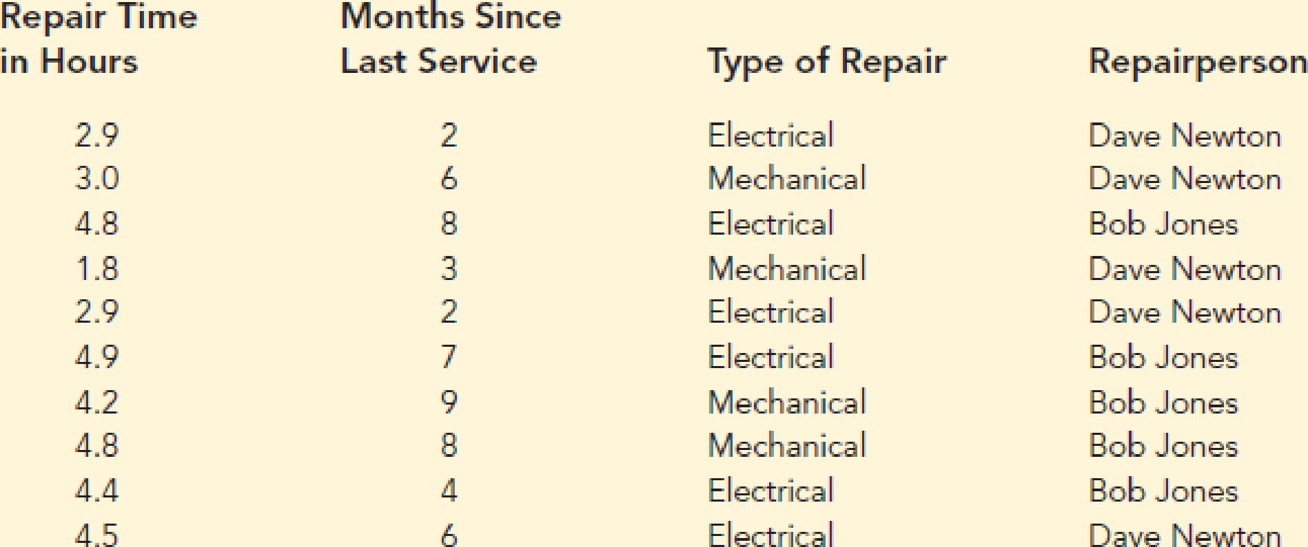
35. Repair Time. Refer to the Johnson Filtration problem introduced in this section. Suppose that in addition to information on the number of months since the machine was serviced and whether a mechanical or an electrical repair was necessary, the managers obtained a list showing which repairperson performed the service. The revised data follow.

1. a. Ignore for now the months since the last maintenance service (x₁) and the repair-person who performed the service. Develop the estimated simple linear regression equation to predict the repair time (y) given the type of repair (x₂). Recall that x₂ = 0 if the type of repair is mechanical and 1 if the type of repair is electrical.
2. b. Does the equation that you developed in part (a) provide a good fit for the observed data? Explain.
3. c. Ignore for now the months since the last maintenance service and the type of repair associated with the machine. Develop the estimated simple linear regression equation to predict the repair time given the repairperson who performed the service. Let x₃ = 0 if Bob Jones performed the service and x₃ = 1 if Dave Newton performed the service.
4. d. Does the equation that you developed in part (c) provide a good fit for the observed data? Explain.