
Videos
Largest University Endowments. University endowments are financial assets that are donated by supporters to be used to provide income to universities. There is a large discrepancy in the size of university endowments. The following table provides a listing of many of the universities that have the largest endowments as reported by the National Association of College and University Business Officers in 2017.
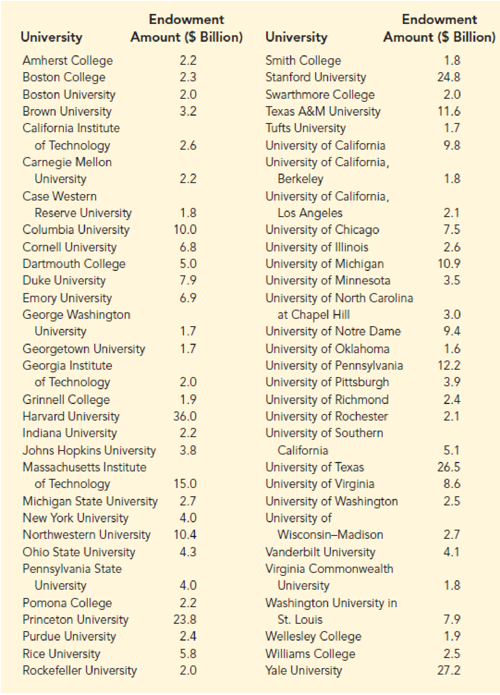
Summarize the data by constructing the following:
- a. A frequency distribution (classes 0–1.9, 2.0–3.9, 4.0–5.9, 6.0–7.9, and so on).
- b. A relative frequency distribution.
- c. A cumulative frequency distribution.
- d. A cumulative relative frequency distribution.
- e. What do these distributions tell you about the endowments of universities?
- f. Show a histogram. Comment on the shape of the distribution.
- g. What is the largest university endowment and which university holds it?
a.
Construct a frequency distribution for the data.
Answer to Problem 21E
The frequency distribution is as follows:
| Endowment Amount ($ Billion) | Frequency |
| 0-1.9 | 10 |
| 2-3.9 | 24 |
| 4-5.9 | 7 |
| 6-7.9 | 5 |
| 8-9.9 | 3 |
| 10-11.9 | 4 |
| 12-13.9 | 1 |
| 14-15.9 | 1 |
| 16-17.9 | 0 |
| 18-19.9 | 0 |
| 20-21.9 | 0 |
| 22-23.9 | 1 |
| 24-25.9 | 1 |
| 26-27.9 | 2 |
| 28-29.9 | 0 |
| 30-31.9 | 0 |
| 32-33.9 | 0 |
| 34-35.9 | 0 |
| 36-37.9 | 1 |
| Total | 60 |
Explanation of Solution
Calculation:
The data represents the Endowment amount of Universities in billions of dollars and the frequency distribution is constructed using the class 0-1.9, 2-3.9, 4-5.9 and so on.
Frequency:
The frequencies are calculated using the tally mark and the range of the data is from 0 to 37.9.
- Based on the given information, the class intervals are 0-1.9, 2-3.9, 4-5.9, …, 36-37.9.
- Make a tally mark for each value in the corresponding revenue class and continue for all values in the data.
- The number of tally marks in each class represents the frequency, f of that class.
Similarly, the frequency of remaining classes for the Endowment is given below:
| Endowment Amount ($ Billion) | Tally | Frequency |
| 0-1.9 | 10 | |
| 2-3.9 | 24 | |
| 4-5.9 | 7 | |
| 6-7.9 | 5 | |
| 8-9.9 | 3 | |
| 10-11.9 | 4 | |
| 12-13.9 | 1 | |
| 14-15.9 | 1 | |
| 16-17.9 | - | 0 |
| 18-19.9 | - | 0 |
| 20-21.9 | - | 0 |
| 22-23.9 | 1 | |
| 24-25.9 | 1 | |
| 26-27.9 | 2 | |
| 28-29.9 | - | 0 |
| 30-31.9 | - | 0 |
| 32-33.9 | - | 0 |
| 34-35.9 | - | 0 |
| 36-37.9 | 1 | |
| Total | 60 |
b.
Construct a relative frequency distribution for the data.
Answer to Problem 21E
The relative frequency distribution is as follows:
| Endowment Amount ($ Billion) | Frequency | Relative frequency |
| 0-1.9 | 10 | 0.17 |
| 2-3.9 | 24 | 0.40 |
| 4-5.9 | 7 | 0.12 |
| 6-7.9 | 5 | 0.08 |
| 8-9.9 | 3 | 0.05 |
| 10-11.9 | 4 | 0.07 |
| 12-13.9 | 1 | 0.02 |
| 14-15.9 | 1 | 0.02 |
| 16-17.9 | 0 | 0.00 |
| 18-19.9 | 0 | 0.00 |
| 20-21.9 | 0 | 0.00 |
| 22-23.9 | 1 | 0.02 |
| 24-25.9 | 1 | 0.02 |
| 26-27.9 | 2 | 0.03 |
| 28-29.9 | 0 | 0.00 |
| 30-31.9 | 0 | 0.00 |
| 32-33.9 | 0 | 0.00 |
| 34-35.9 | 0 | 0.00 |
| 36-37.9 | 1 | 0.02 |
| Total | 60 | 1 |
Explanation of Solution
Calculation:
Relative frequency:
The general formula for the relative frequency is given below:
For the class (0-1.9), substitute frequency as “10” and total frequency as “60”.
Similarly, the relative frequencies for the remaining Endowment classes are obtained below:
| Endowment Amount ($ Billion) | Frequency | Relative frequency |
| 0-1.9 | 10 | 0.17 |
| 2-3.9 | 24 | 0.40 |
| 4-5.9 | 7 | 0.12 |
| 6-7.9 | 5 | 0.08 |
| 8-9.9 | 3 | 0.05 |
| 10-11.9 | 4 | 0.07 |
| 12-13.9 | 1 | 0.02 |
| 14-15.9 | 1 | 0.02 |
| 16-17.9 | 0 | 0.00 |
| 18-19.9 | 0 | 0.00 |
| 20-21.9 | 0 | 0.00 |
| 22-23.9 | 1 | 0.02 |
| 24-25.9 | 1 | 0.02 |
| 26-27.9 | 2 | 0.03 |
| 28-29.9 | 0 | 0.00 |
| 30-31.9 | 0 | 0.00 |
| 32-33.9 | 0 | 0.00 |
| 34-35.9 | 0 | 0.00 |
| 36-37.9 | 1 | 0.02 |
| Total | 60 | 1 |
c.
Construct a cumulative frequency distribution for the data.
Answer to Problem 21E
The cumulative frequency distribution is as follows:
| Endowment Amount ($ Billion) | Frequency | Cumulative frequency |
| 0-1.9 | 10 | 10 |
| 2-3.9 | 24 | 34 |
| 4-5.9 | 7 | 41 |
| 6-7.9 | 5 | 46 |
| 8-9.9 | 3 | 49 |
| 10-11.9 | 4 | 53 |
| 12-13.9 | 1 | 54 |
| 14-15.9 | 1 | 55 |
| 16-17.9 | 0 | 55 |
| 18-19.9 | 0 | 55 |
| 20-21.9 | 0 | 55 |
| 22-23.9 | 1 | 56 |
| 24-25.9 | 1 | 57 |
| 26-27.9 | 2 | 59 |
| 28-29.9 | 0 | 59 |
| 30-31.9 | 0 | 59 |
| 32-33.9 | 0 | 59 |
| 34-35.9 | 0 | 59 |
| 36-37.9 | 1 | 60 |
Explanation of Solution
Calculation:
Cumulative frequency:
Cumulative frequency of a particular class is the sum of all frequencies up to that class. The last class’s cumulative frequency is equal to the sample size
Thus, the cumulative frequencies for the endowment classes are obtained below:
| Endowment Amount ($ Billion) | Frequency | Cumulative frequency |
| 0-1.9 | 10 | 10 |
| 2-3.9 | 24 | |
| 4-5.9 | 7 | |
| 6-7.9 | 5 | |
| 8-9.9 | 3 | |
| 10-11.9 | 4 | |
| 12-13.9 | 1 | |
| 14-15.9 | 1 | |
| 16-17.9 | 0 | |
| 18-19.9 | 0 | |
| 20-21.9 | 0 | |
| 22-23.9 | 1 | |
| 24-25.9 | 1 | |
| 26-27.9 | 2 | |
| 28-29.9 | 0 | |
| 30-31.9 | 0 | |
| 32-33.9 | 0 | |
| 34-35.9 | 0 | |
| 36-37.9 | 1 |
d.
Construct a cumulative relative frequency distribution for the data.
Answer to Problem 21E
The cumulative relative frequency distribution is given below:
| Endowment Amount ($ Billion) | Frequency | Cumulative Relative Frequency |
| 0-1.9 | 10 | 0.17 |
| 2-3.9 | 24 | 0.57 |
| 4-5.9 | 7 | 0.69 |
| 6-7.9 | 5 | 0.77 |
| 8-9.9 | 3 | 0.82 |
| 10-11.9 | 4 | 0.89 |
| 12-13.9 | 1 | 0.90 |
| 14-15.9 | 1 | 0.92 |
| 16-17.9 | 0 | 0.92 |
| 18-19.9 | 0 | 0.92 |
| 20-21.9 | 0 | 0.92 |
| 22-23.9 | 1 | 0.94 |
| 24-25.9 | 1 | 0.95 |
| 26-27.9 | 2 | 0.99 |
| 28-29.9 | 0 | 0.99 |
| 30-31.9 | 0 | 0.99 |
| 32-33.9 | 0 | 0.99 |
| 34-35.9 | 0 | 0.99 |
| 36-37.9 | 1 | 1.00 |
Explanation of Solution
Calculation:
Cumulative relative frequency of a particular class is the sum of all relative frequencies up to that class. The last class’s cumulative relative frequency is equal to the approximate value 1.00.
The relative frequencies for the endowment classes from part (b) is given below:
| Endowment Amount ($ Billion) | Frequency | Relative frequency |
| 0-1.9 | 10 | 0.17 |
| 2-3.9 | 24 | 0.40 |
| 4-5.9 | 7 | 0.12 |
| 6-7.9 | 5 | 0.08 |
| 8-9.9 | 3 | 0.05 |
| 10-11.9 | 4 | 0.07 |
| 12-13.9 | 1 | 0.02 |
| 14-15.9 | 1 | 0.02 |
| 16-17.9 | 0 | 0.00 |
| 18-19.9 | 0 | 0.00 |
| 20-21.9 | 0 | 0.00 |
| 22-23.9 | 1 | 0.02 |
| 24-25.9 | 1 | 0.02 |
| 26-27.9 | 2 | 0.03 |
| 28-29.9 | 0 | 0.00 |
| 30-31.9 | 0 | 0.00 |
| 32-33.9 | 0 | 0.00 |
| 34-35.9 | 0 | 0.00 |
| 36-37.9 | 1 | 0.02 |
| Total | 60 | 1 |
Thus, the cumulative relative frequencies for the endowment classes are obtained below:
| Endowment Amount ($ Billion) | Relative frequency | Cumulative Relative Frequency |
| 0-1.9 | 0.17 | 0.17 |
| 2-3.9 | 0.40 | |
| 4-5.9 | 0.12 | |
| 6-7.9 | 0.08 | |
| 8-9.9 | 0.05 | |
| 10-11.9 | 0.07 | |
| 12-13.9 | 0.02 | |
| 14-15.9 | 0.02 | |
| 16-17.9 | 0.00 | |
| 18-19.9 | 0.00 | |
| 20-21.9 | 0.00 | |
| 22-23.9 | 0.02 | |
| 24-25.9 | 0.02 | |
| 26-27.9 | 0.03 | |
| 28-29.9 | 0.00 | |
| 30-31.9 | 0.00 | |
| 32-33.9 | 0.00 | |
| 34-35.9 | 0.00 | |
| 36-37.9 | 0.02 | 1.00 |
e.
Explain about the endowment of universities using the distributions.
Explanation of Solution
From the given data set and obtained distributions , it is observed that the frequency for the endowment of universities in the range of 0 billion dollars to less than $16 billion dollars is obtained by majority of 55 Universities over 60 Universities.
Further, the endowment of universities greater $16 billion is obtained by only 5 Universities.
Moreover, 92% of universities have endowment amount under 16 billion dollars. Only 8% of universities have endowment amount over 16 billion dollars.
f.
Construct the histogram and comment on the shape of the distribution.
Answer to Problem 21E
- Output using Excel is given below:
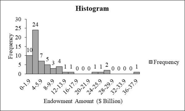
The histogram is skewed to the right.
Explanation of Solution
Calculation:
Step-by-step procedure to draw the frequency histogram chart using Excel is as follows:
- In Excel sheet, enter Endowment Amount ($ Billion) in one column and Frequency in another column.
- Select the data and then choose Insert > Insert Column Bar Charts.
- Select Clustered Column Under More Column Charts.
- Double click the bars
- In Format Data Series, enter 0 in Gap Width under Series Options.
Skewness:
The data is said to be skewed if there is lack of symmetry and values fall on one side that is, either left or right of the distribution.
Right skewed:
If the tail on the distribution is elongated toward the right, more over it attains its peak rapidly than its horizontal axis and then it is a right skewed distribution. It is also called positively skewed.
The distribution of Endowment in the histogram has elongated tail toward right side. There are five universities in the range 20 billion dollars to 37.9 billion dollars.
Therefore, the distribution of the histogram with Endowment is skewed right.
g.
Find the largest university endowment and find the university that holds the largest endowment.
Answer to Problem 21E
The largest university endowment is $36 billion.
The University H holds the largest endowment.
Explanation of Solution
From the data set of 60 universities, it is observed that the largest university endowment is $36 billion and the university is University H.
Moreover, the endowment of remaining universities has less than 28 billion dollars and most of the universities have less than 16 billion dollars and is approximately 92 percent.
Want to see more full solutions like this?
Chapter 2 Solutions
Essentials Of Statistics For Business & Economics


 Glencoe Algebra 1, Student Edition, 9780079039897...AlgebraISBN:9780079039897Author:CarterPublisher:McGraw Hill