
Introductory Statistics (10th Edition)
10th Edition
ISBN: 9780321989178
Author: Neil A. Weiss
Publisher: PEARSON
expand_more
expand_more
format_list_bulleted
Concept explainers
Videos
Textbook Question
Chapter 2.4, Problem 151E
SnowGoose Nests. In the article “Trophic Interaction Cycles in Tundra Ecosystems and the Impact of Climate Change” (Bio- Science, Vol. 55, No. 4, pp. 311–321), R. Ims and E. Fuglei provided an overview of animal species in the northern tundra. One threat to the snow goose in arctic Canada is the lemming. Snowy owls act as protection to the snow goose breeding grounds. For two years that are 3 years apart, the following graphs give relative frequency histograms of the distances, in meters, of snow goose nests to the nearest snowy owl nest.
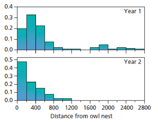
For each histogram, do the following:
- a. Identify the shape of the distribution with regard to modality.
- b. Identify the shape of the distribution with regard to symmetry (or nonsymmetry).
- c. If the distribution is unimodal and nonsymmetric, classify it as either right skewed or left skewed.
- d. Compare the two distributions.
Expert Solution & Answer
Want to see the full answer?
Check out a sample textbook solution
Students have asked these similar questions
PCBs and Pelicans. Polychlorinated biphenyls (PCBs), industrial pollutants, are known to be carcinogens and a great danger to natural ecosystems. As a result of several studies, PCB production was banned in the United States in 1979 and by the Stockholm Convention on Persistent Organic Pollutants in 2001. One study, published in 1972 by R. Risebrough, is titled “Effects of Environmental Pollutants Upon Animals Other Than Man” (Proceedings of the 6th Berkeley Symposium on Mathematics and Statistics, VI, University of California Press, pp. 443–463). In that study, 60 Anacapa pelican eggs were collected and measured for their shell thickness, in millimeters (mm), and concentration of PCBs, in parts per million (ppm). The data are on the WeissStats site.
a. obtain and interpret the standard error of the estimate.
b. obtain a residual plot and a normal probability plot of the residuals.
c. decide whether you can reasonably consider Assumptions 1–3 for regression inferences met by the two…
PCBs and Pelicans. Polychlorinated biphenyls (PCBs), industrial pollutants, are known to be carcinogens and a great danger to natural ecosystems. As a result of several studies, PCB production was banned in the United States in 1979 and by the Stockholm Convention on Persistent Organic Pollutants in 2001. One study, published in 1972 by R. W. Risebrough, is titled ‘‘Effects of Environmental Pollutants Upon Animals Other Than Man’’ (Proceedings of the 6th Berkeley Symposium on Mathematics and Statistics, VI, University of California Press, pp. 443–463). In that study, 60 Anacapa pelican eggs were collected and measured for their shell thickness, in millimeters (mm), and concentration of PCBs, in parts per million (ppm). Following is a relative-frequency histogram of the PCB concentration data.
For 25 years, Arthur Reynolds and Judy Temple tracked more than 1,400 children who participated in a publicly funded early childhood development program beginning at age 3. They found that children who participated in the program showed higher levels of educational attainment, socioeconomic status, and job skills, as well as lower rates of substance abuse, felony arrest, and incarceration, than those who did not receive school-based early education. One possible theory for the success of this program is that improving school readiness improved the children's success in school. The improved success in school in turn improved their readiness for adulthood, resulting in increased job skills and socioeconomic status as well as lower rates of substance abuse.
What is the independent and dependent variable?
Chapter 2 Solutions
Introductory Statistics (10th Edition)
Ch. 2.1 - Give an example, other than those presented in...Ch. 2.1 - Explain the meaning of a. qualitative variable. b....Ch. 2.1 - Explain the meaning of a. qualitative data. b....Ch. 2.1 - Provide a reason why the classification of data is...Ch. 2.1 - Of the variables you have studied so far, which...Ch. 2.1 - For each part of Exercises 2.62.11, classify the...Ch. 2.1 - Earthquakes. The U.S. Geological Survey monitors...Ch. 2.1 - Top 10 IPOs. An online article from the Washington...Ch. 2.1 - Earnings from the Crypt. On the Celebrity NetWorth...Ch. 2.1 - World University Rankings. The Times Higher...
Ch. 2.1 - Recording Industry Statistics. The Recording...Ch. 2.1 - RBI Kings. As reported on MLB.com, the five...Ch. 2.1 - Top Broadcast Shows. As reported in Primetime...Ch. 2.1 - The Fulbright Program. The U.S. governments...Ch. 2.1 - Top 10 Green Cars. The following table presents...Ch. 2.1 - Ordinal Data. Another important type of data is...Ch. 2.2 - What is a frequency distribution of qualitative...Ch. 2.2 - Explain the difference between a. frequency and...Ch. 2.2 - Answer true or false to each of the statements in...Ch. 2.2 - In Exercises 2.202.25, we have presented some...Ch. 2.2 - Prob. 21ECh. 2.2 - In Exercises 2.202.25, we have presented some...Ch. 2.2 - Prob. 23ECh. 2.2 - In Exercises 2.202.25, we have presented some...Ch. 2.2 - In Exercises 2.202.25, we have presented some...Ch. 2.2 - For each data set in Exercises 2.262.31, a....Ch. 2.2 - For each data set in Exercises 2.262.31, a....Ch. 2.2 - For each data set in Exercises 2.262.31, a....Ch. 2.2 - For each data set in Exercises 2.262.31, a....Ch. 2.2 - For each data set in Exercises 2.262.31, a....Ch. 2.2 - For each data set in Exercises 2.262.31, a....Ch. 2.2 - In each of Exercises 2.322.37, we have presented a...Ch. 2.2 - In each of Exercises 2.322.37, we have presented a...Ch. 2.2 - In each of Exercises 2.322.37, we have presented a...Ch. 2.2 - In each of Exercises 2.322.37, we have presented a...Ch. 2.2 - In each of Exercises 2.322.37, we have presented a...Ch. 2.2 - Prob. 37ECh. 2.2 - Health Status. The National Center for Health...Ch. 2.2 - In Exercises 2.392.41, use the technology of your...Ch. 2.2 - Prob. 40ECh. 2.2 - In Exercises 2.392.41, use the technology of your...Ch. 2.3 - Identify an important reason for grouping data.Ch. 2.3 - Do the concepts of class limits, marks, cutpoints,...Ch. 2.3 - State three of the most important guidelines in...Ch. 2.3 - With regard to grouping quantitative data into...Ch. 2.3 - For quantitative data, we examined three types of...Ch. 2.3 - We used slightly different methods for determining...Ch. 2.3 - Explain the difference between a frequency...Ch. 2.3 - Explain the advantages and disadvantages of...Ch. 2.3 - For data that are grouped in classes based on more...Ch. 2.3 - Discuss the relative advantages and disadvantages...Ch. 2.3 - Suppose that you have a data set that contains a...Ch. 2.3 - Suppose that you have constructed a stem-and-leaf...Ch. 2.3 - In each of Exercises 2.542.59, we have presented a...Ch. 2.3 - In each of Exercises 2.542.59, we have presented a...Ch. 2.3 - In each of Exercises 2.542.59, we have presented a...Ch. 2.3 - In each of Exercises 2.542.59, we have presented a...Ch. 2.3 - Prob. 58ECh. 2.3 - In each of Exercises 2.542.59, we have presented a...Ch. 2.3 - Prob. 60ECh. 2.3 - Prob. 61ECh. 2.3 - In Exercises 2.602.71, we have presented some...Ch. 2.3 - In Exercises 2.602.71, we have presented some...Ch. 2.3 - In Exercises 2.602.71, we have presented some...Ch. 2.3 - In Exercises 2.602.71, we have presented some...Ch. 2.3 - Prob. 66ECh. 2.3 - In Exercises 2.602.71, we have presented some...Ch. 2.3 - In Exercises 2.602.71, we have presented some...Ch. 2.3 - Prob. 69ECh. 2.3 - In Exercises 2.602.71, we have presented some...Ch. 2.3 - In Exercises 2.602.71, we have presented some...Ch. 2.3 - Prob. 72ECh. 2.3 - In each of Exercises 2.722.75, construct a dotplot...Ch. 2.3 - Prob. 74ECh. 2.3 - In each of Exercises 2.722.75, construct a dotplot...Ch. 2.3 - In each of Exercises 2.762.79, construct a...Ch. 2.3 - Prob. 77ECh. 2.3 - In each of Exercises 2.762.79, construct a...Ch. 2.3 - Prob. 79ECh. 2.3 - Prob. 80ECh. 2.3 - For each data set in Exercises 2.802.91, use the...Ch. 2.3 - For each data set in Exercises 2.802.91, use the...Ch. 2.3 - For each data set in Exercises 2.802.91, use the...Ch. 2.3 - For each data set in Exercises 2.802.91, use the...Ch. 2.3 - For each data set in Exercises 2.802.91, use the...Ch. 2.3 - For each data set in Exercises 2.802.91, use the...Ch. 2.3 - Prob. 87ECh. 2.3 - Prob. 88ECh. 2.3 - Prob. 89ECh. 2.3 - Prob. 90ECh. 2.3 - Prob. 91ECh. 2.3 - Prob. 92ECh. 2.3 - Age of Passenger Cars. According to R. L. Polk ...Ch. 2.3 - Stressed-Out Bus Drivers. Frustrated passengers,...Ch. 2.3 - Acute Postoperative Days. Several neurosurgeons...Ch. 2.3 - MMs. In the article Sweetening StatisticsWhat MMs...Ch. 2.3 - Women in the Workforce. In an issue of Science...Ch. 2.3 - Process Capability. R. Morris and E. Watson...Ch. 2.3 - University Patents. The number of patents a...Ch. 2.3 - Prob. 100ECh. 2.3 - Prob. 101ECh. 2.3 - Adjusted Gross Incomes. The Internal Revenue...Ch. 2.3 - Cholesterol Levels. According to the National...Ch. 2.3 - Hospital Beds. The number of hospital beds...Ch. 2.3 - Parkinsons Disease. Parkinsons disease affects...Ch. 2.3 - The Great White Shark. In an article titled Great...Ch. 2.3 - The Beatles. In the article, Length of The Beatles...Ch. 2.3 - High School Completion. As reported by the U.S....Ch. 2.3 - Prob. 109ECh. 2.3 - Body Temperature. A study by researchers at the...Ch. 2.3 - Exam Scores. The exam scores for the students in...Ch. 2.3 - Prob. 112ECh. 2.3 - Prob. 113ECh. 2.3 - Age and Gender. The following bivariate data on...Ch. 2.3 - Prob. 115ECh. 2.3 - Clocking the Cheetah. Construct a...Ch. 2.3 - Prob. 117ECh. 2.3 - Residential Energy Consumption. Refer to the...Ch. 2.3 - Prob. 119ECh. 2.3 - Cardiovascular Hospitalizations. The Florida State...Ch. 2.3 - Prob. 121ECh. 2.4 - In each of Exercises 2.1222.127, explain the...Ch. 2.4 - In each of Exercises 2.1222.127, explain the...Ch. 2.4 - In each of Exercises 2.1222.127, explain the...Ch. 2.4 - Prob. 125ECh. 2.4 - Prob. 126ECh. 2.4 - Prob. 127ECh. 2.4 - Prob. 128ECh. 2.4 - Suppose that a variable of a population has a...Ch. 2.4 - Prob. 130ECh. 2.4 - Identify and sketch three distribution shapes that...Ch. 2.4 - Prob. 132ECh. 2.4 - In each of Exercises 2.1322.139, we have drawn a...Ch. 2.4 - In each of Exercises 2.1322.139, we have drawn a...Ch. 2.4 - In each of Exercises 2.1322.139, we have drawn a...Ch. 2.4 - In each of Exercises 2.1322.139, we have drawn a...Ch. 2.4 - In each of Exercises 2.1322.139, we have drawn a...Ch. 2.4 - In each of Exercises 2.1322.139, we have drawn a...Ch. 2.4 - Prob. 139ECh. 2.4 - In each of Exercises 2.1402.149, we have provided...Ch. 2.4 - In each of Exercises 2.1402.149, we have provided...Ch. 2.4 - Prob. 142ECh. 2.4 - In each of Exercises 2.1402.149, we have provided...Ch. 2.4 - In each of Exercises 2.1402.149, we have provided...Ch. 2.4 - In each of Exercises 2.1402.149, we have provided...Ch. 2.4 - In each of Exercises 2.1402.149, we have provided...Ch. 2.4 - Prob. 147ECh. 2.4 - Prob. 148ECh. 2.4 - Prob. 149ECh. 2.4 - Old Faithful. Old Faithful is a geyser in...Ch. 2.4 - SnowGoose Nests. In the article Trophic...Ch. 2.4 - Prob. 152ECh. 2.4 - In each of Exercises 2.1522.157, a. use the...Ch. 2.4 - In each of Exercises 2.1522.157, a. use the...Ch. 2.4 - Prob. 155ECh. 2.4 - In each of Exercises 2.1522.157, a. use the...Ch. 2.4 - In each of Exercises 2.1522.157, a. use the...Ch. 2.4 - Standard Normal Distribution. One of the most...Ch. 2.5 - Give one reason why constructing and reading...Ch. 2.5 - Prob. 163ECh. 2.5 - Reading Skills. Each year the director of the...Ch. 2.5 - Americas Melting Pot. The U.S. Census Bureau...Ch. 2.5 - Prob. 167ECh. 2.5 - Drunk-Driving Fatalities. Drunk-driving fatalities...Ch. 2.5 - Prob. 169ECh. 2.5 - Prob. 170ECh. 2.5 - Prob. 171ECh. 2 - This problem is about variables. a. What is a...Ch. 2 - This problem is about data. a. What are data? b....Ch. 2 - For a qualitative data set, what is a a. frequency...Ch. 2 - What is the relationship between a frequency or...Ch. 2 - Identify two main types of graphical displays that...Ch. 2 - In a bar chart, unlike in a histogram, the bars do...Ch. 2 - Some users of statistics prefer pie charts to bar...Ch. 2 - When is the use of single-value grouping...Ch. 2 - A quantitative data set has been grouped by using...Ch. 2 - A quantitative data set has been grouped by using...Ch. 2 - A quantitative data set has been grouped by using...Ch. 2 - A quantitative data set has been grouped by using...Ch. 2 - Explain the relative positioning of the bars in a...Ch. 2 - Sketch the curve corresponding to each of the...Ch. 2 - Draw a smooth curve that represents a symmetric...Ch. 2 - Prob. 16RPCh. 2 - Largest Hydroelectric Plants. According to...Ch. 2 - DVD Players. Refer to Example 2.16 on page 60. a....Ch. 2 - Inauguration Ages. From the Information Please...Ch. 2 - Inauguration Ages. Refer to Problem 19. Construct...Ch. 2 - Prob. 21RPCh. 2 - Prob. 22RPCh. 2 - Busy Bank Tellers. The Prescott National Bank has...Ch. 2 - On-Time Arrivals. The Air Travel Consumer Report...Ch. 2 - Old Ballplayers. From the ESPN Web site, we...Ch. 2 - Prob. 26RPCh. 2 - U.S. Divisions. The U.S. Census Bureau divides the...Ch. 2 - Prob. 28RPCh. 2 - Prob. 29RPCh. 2 - Hair and Eye Color. In the article Graphical...Ch. 2 - Prob. 31RPCh. 2 - In Problems 3133, a. identify the population and...Ch. 2 - In Problems 3133, a. identify the population and...Ch. 2 - UWEC UNDERGRADUATES Recall from Chapter 1 (see...Ch. 2 - Recall that, each year, Forbes magazine publishes...
Knowledge Booster


Learn more about
Need a deep-dive on the concept behind this application? Look no further. Learn more about this topic, statistics and related others by exploring similar questions and additional content below.Similar questions
- The extending research findings and conclusions from a study conducted on a sample population to the population at large is called? Transferability Generalizability Causality All of the abovearrow_forwardA local church is interested in determining how length of residence in the present community relates to church attendance. Using a random sample of 15 individuals, they gathered data on how many times in the previous 5 weeks each individual attended church services. The data are provided below. Length of residence in the community Less than 2 years 2-5 years More than 5 years 0 0 1 1 2 3 3 3 3 4 4 4 4 5 4 Using the 5-step model, determine whether and how church attendance is related to length of residence in the community. Use 5% and 1% levels of statistical significance. What are the assumptions for this problem?arrow_forwardHere is a dataset containing plant growth measurements of plants grown in solutions of commonly-found chemicals in roadway runoff.Phragmites australis, a fast-growing non-native grass common to roadsides and disturbed wetlands of Tidewater Virginia, was grown in a greenhouse and watered with either: Distilled water (control); A weak petroleum solution (representing standard roadway runoff); Sodium chloride solution; Magnesium chloride solution; De-icing brine (50% sodium chloride and 50% magnesium chloride).Twenty grass preparations were used for each solution, and total growth (in cm) was recorded after watering every other day for 40 days.-Perform the correct statistical test to determine the p-value.-Report your answer rounded to four decimal places.-You should use formulas, functions, and the Data Analysis ToolPak in MS Excel to avoid additive rounding errors. Here are some useful functions: =t.test(array1,array2,tails,type) Produces a p-value for any…arrow_forward
- Reference: Camm J.D. et al., (2019) Business Analytics: descriptive, predictive and prescriptive (3rd edition). Cengage ____________________________________________________________________________________ Jay Gatsby categorizes wines into one of three clusters. The centroids of these clusters, describing the average characteristics of a wine in each cluster, are listed in the following table. Characteristic Cluster 1 Cluster 2 Cluster 3 Alcohol 0.819 0.164 -0.937 MalicAcid -0.329 0.869 -0.368 Ash 0.248 0.186 -0.393 Alcalinity…arrow_forwardIn a study of exhaust emissions from school buses, the pollution intake by passengers was determined for a sample of nine school buses used in the Southern California Air Basin. The pollution intake is the amount of exhaust emissions, in grams per person per million grams emitted, that would be inhaled while traveling on the bus during its usual 18-mile18-mile trip on congested freeways from South Central LA to a magnet school in West LA. (In comparison, a city of 11 million people will inhale a total of about 1212 grams of exhaust per million grams emitted.) The amounts for the nine buses when driven with the windows open are given in the table. 1.15 0.33 0.40 0.33 1.35 0.38 0.25 0.40 0.35 A good way to judge the effect of outliers is to do your analysis twice, once with the outliers and a second time without them. Give the 90%90% confidence interval with all the data for the mean pollution intake among all school buses used in the Southern California Air Basin that…arrow_forwardDefine A Competitive-Hunter Model ?arrow_forward
- A researcher wants to determine the causal relationship among number of family members who are at least high school graduate (W), number of working family members (X), monthly gross income (Y), monthly expenditure (Z), and average monthly bank deposits (A). A random sample of 20 families was selected and the data on the variables were collected (see household.xslx). Consider the following path diagram: 1. Set-up the structural equations. Consider the R outputs from the conducted path analysis. 2. Identify the factors affecting the endogenous variables. Leave blank if variable is exogenous. W: ____________ X: ____________ Y: ____________ Z: ____________ A: ____________ 3. Illustrate the output path diagram including the estimated path coefficients.arrow_forwardSecond-Hand Smoke: Data Set 12 “Passive and Active Smoke” in Appendix B includes cotinine levels measured in a group of nonsmokers exposed to tobacco smoke (n = 40, Mean = 60.58 ng>mL, s = 138.08 ng>mL) and a group of nonsmokers not exposed to tobacco smoke (n = 40, Mean = 16.35 ng>mL, s = 62.53 ng>mL). Cotinine is a metabolite of nicotine, meaning that when nicotine is absorbed by the body, cotinine is produced. Use a 0.05 significance level to test the claim that nonsmokers exposed to tobacco smoke have a higher mean cotinine level than nonsmokers not exposed to tobacco smoke. Construct the confidence interval appropriate for the hypothesis test in part a. What do you conclude about the effects of second-hand smoke?arrow_forwardA research group is interested in the relationship between exposure to mold in households after a major hurricane and the onset of acute respiratory illness in children. Suppose an observational study is conducted over 10 years following the natural disaster and the following two-by-two table was created in order to address the relationship between exposure and outcome. Acute Respiratory Illness No Acute Respiratory Illness Total Mold 378 156 534 No Mold 73 260 333 Total 451 416 867 Calculate the incidence of acute respiratory illness in the exposed and unexposed. Calculate the relative risk for ARI due to exposure in this study Interpret your findings from part Barrow_forward
- Exercise 13-4 (LO13-2) The production department of Celltronics International wants to explore the relationship between the number of employees who assemble a subassembly and the number produced. As an experiment, two employees were assigned to assemble the subassemblies. They produced 15 during a one-hour period. Then four employees assembled them. They produced 25 during a one-hour period. The complete set of paired observations follows. Number ofAssemblers One-HourProduction (units) 2 15 4 25 1 10 5 40 3 30 The dependent variable is production; that is, it is assumed that different levels of production result from a different number of employees. Draw a scatter diagram. Please state exact coordinates Based on the scatter diagram, does there appear to be any relationship between the number of assemblers and production? Compute the coefficient correlation. (Negative values should be…arrow_forward5. A consumer buying cooperative tested the effective heating area of 20 different electric space heaters with different wattages. Here are the results. Heater Wattage Area 1 750 291 2 1,750 83 3 1,250 215 4 1,750 209 5 1,500 295 6 750 153 7 1,000 40 8 750 166 9 1,250 115 10 1,250 146 11 750 113 12 1,000 56 13 1,750 284 14 1,000 45 15 750 82 16 1,250 175 17 750 150 18 1,500 231 19 1,000 87 20 750 52 Click here for the Excel Data FileRequired:a. Compute the correlation between the wattage and heating area. Is there a direct or an indirect relationship? (Round your answer to 4 decimal places.) b. Conduct a test of hypothesis to determine if it is reasonable that the coefficient is greater than zero. Use the 0.050 significance level. (Round intermediate calculations and final answer to 3 decimal places.)H0: ρ ≤ 0; H1: ρ > 0 Reject H0 if t > 1.734…arrow_forwardReview Question 18arrow_forward
arrow_back_ios
SEE MORE QUESTIONS
arrow_forward_ios
Recommended textbooks for you
 MATLAB: An Introduction with ApplicationsStatisticsISBN:9781119256830Author:Amos GilatPublisher:John Wiley & Sons Inc
 Probability and Statistics for Engineering and th...StatisticsISBN:9781305251809Author:Jay L. DevorePublisher:Cengage Learning
 Statistics for The Behavioral Sciences (MindTap C...StatisticsISBN:9781305504912Author:Frederick J Gravetter, Larry B. WallnauPublisher:Cengage Learning
 Elementary Statistics: Picturing the World (7th E...StatisticsISBN:9780134683416Author:Ron Larson, Betsy FarberPublisher:PEARSON
 The Basic Practice of StatisticsStatisticsISBN:9781319042578Author:David S. Moore, William I. Notz, Michael A. FlignerPublisher:W. H. Freeman
 Introduction to the Practice of StatisticsStatisticsISBN:9781319013387Author:David S. Moore, George P. McCabe, Bruce A. CraigPublisher:W. H. Freeman
MATLAB: An Introduction with Applications
Statistics
ISBN:9781119256830
Author:Amos Gilat
Publisher:John Wiley & Sons Inc
Probability and Statistics for Engineering and th...
Statistics
ISBN:9781305251809
Author:Jay L. Devore
Publisher:Cengage Learning
Statistics for The Behavioral Sciences (MindTap C...
Statistics
ISBN:9781305504912
Author:Frederick J Gravetter, Larry B. Wallnau
Publisher:Cengage Learning
Elementary Statistics: Picturing the World (7th E...
Statistics
ISBN:9780134683416
Author:Ron Larson, Betsy Farber
Publisher:PEARSON
The Basic Practice of Statistics
Statistics
ISBN:9781319042578
Author:David S. Moore, William I. Notz, Michael A. Fligner
Publisher:W. H. Freeman
Introduction to the Practice of Statistics
Statistics
ISBN:9781319013387
Author:David S. Moore, George P. McCabe, Bruce A. Craig
Publisher:W. H. Freeman
Hypothesis Testing - Solving Problems With Proportions; Author: The Organic Chemistry Tutor;https://www.youtube.com/watch?v=76VruarGn2Q;License: Standard YouTube License, CC-BY
Hypothesis Testing and Confidence Intervals (FRM Part 1 – Book 2 – Chapter 5); Author: Analystprep;https://www.youtube.com/watch?v=vth3yZIUlGQ;License: Standard YouTube License, CC-BY