
Concept explainers
Videos
Household Incomes. The following data represent a sample of 14 household incomes ($1000s). Answer the following questions based on this sample.

- a. What is the median household income for these sample data?
- b. According to a previous survey, the median annual household income five years ago was $55,000. Based on the sample data above, estimate the percentage change in the median household income from five years ago to today.
- c. Compute the first and third
quartiles . - d. Provide a five-number summary.
- e. Using the z-score approach, do the data contain any outliers? Does the approach that uses the values of the first and third quartiles and the
interquartile range to detect outliers provide the same results?
a.
Find the median household income for the given sample.
Answer to Problem 68SE
The median household income for the given sample is $52,100.
Explanation of Solution
Calculation:
The data represent the incomes (in $1,000s) for a sample of 14 households. Five years ago the median annual household income was $55,500.
Software procedure:
Step by step procedure to obtain the descriptive statistics using EXCEL is as follows:
- In an EXCEL sheet enter the values of the sample and label it as Sample.
- Go to Data > Data Analysis (in case it is not default, take the Analysis ToolPak from Excel Add Ins) > Descriptive statistics.
- Enter Input Range as $A$2:$A$15, select Columns in Grouped By, tick on Summary statistics.
- Click on OK.
Output using EXCEL is given as follows:
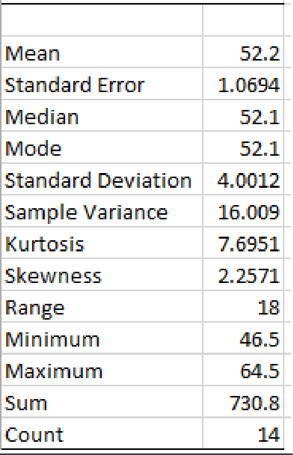
From the EXCEL output, the median is 52.1.
Thus, the median household income for the given sample is $52,100.
b.
Find the percentage change in the median household income from five years ago to today.
Answer to Problem 68SE
The percentage change in the median household income from five years ago to today is decreased by 6.1%.
Explanation of Solution
Calculation:
Five years ago, the median annual household income was $55,500 (55.5).
The median household income for the given sample is $52,100 (52.1).
The percentage change in the median household income from five years ago to today can be obtained as given below:
Thus, the percentage change in the median household income from five years ago to today is decreased by 6.1%.
c.
Find the first and third quartiles.
Answer to Problem 68SE
The first and third quartiles are 50.75, and 52.6, respectively.
Explanation of Solution
Calculation:
First quartile:
The EXCEL function to compute first quartile is
Software Procedure:
Step by step procedure to obtain the first quartile using EXCEL is as follows:
- Open an EXCEL file.
- Enter the data in the column J in cells J1 to J14.
- In a cell A1, enter the formula QUARTILE.EXC (J1:J14,1).
- Click on OK.
Output using EXCEL is given as follows:
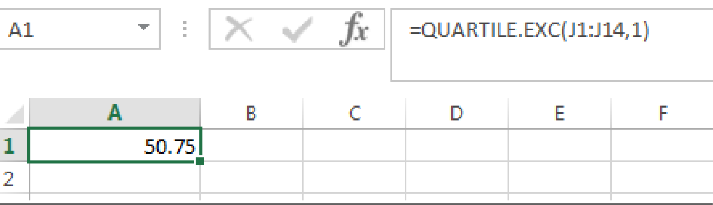
From the EXCEL output, the first quartile of the sample data is 50.75.
Third quartile:
The EXCEL function to compute third quartile is
Software Procedure:
Step by step procedure to obtain the third quartile using EXCEL is as follows:
- Open an EXCEL file.
- Enter the data in the column J in cells J1 to J14.
- In a cell A1, enter the formula QUARTILE.EXC (J1:J14,3).
- Click on OK.
Output using EXCEL is given as follows:
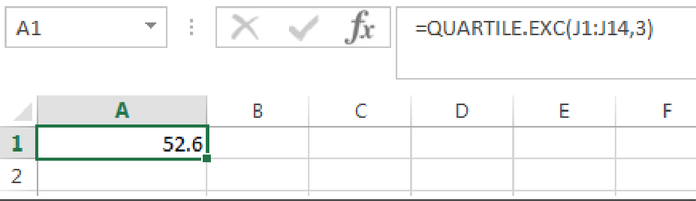
From the EXCEL output, the third quartile of the sample data is 52.6.
Thus, the first and third quartiles are 50.75, and 52.6, respectively.
d.
Find the five number summary for the data.
Answer to Problem 68SE
The five-number summary of the data is 46.5, 50.75, 52.1, 52.6 and 64.5.
Explanation of Solution
Calculation:
The five number summary consists the values of minimum, first quartile, second quartile, third quartile, maximum.
From the EXCEL output obtained in Part (a), the maximum, median, and minimum values are 64.5, and 46.5, respectively.
From Part (c), the first and third quartiles of the dataset are 50.75 and 52.6, respectively.
The quartiles of the data set are
Thus, the five-number summary of the dataset is given below:
- Minimum: 46.5,
- First quartile: 50.75,
- Median: 52.1,
- Third quartile: 52.6,
- Maximum: 64.5.
e.
Check for the outliers in the dataset by using the z-score approach.
Check for the outliers in the dataset by using quartiles and interquartile range.
Check whether or not result obtained using z-score approach matches with the result obtained using quartiles and interquartile range.
Answer to Problem 68SE
The outlier using z-score approach is 64.5.
The outliers using quartiles and interquartile range are 49.4, and 64.5.
The result obtained using z-score approach does not matches with the result obtained using quartiles and interquartile range.
Explanation of Solution
Calculation:
From the EXCEL output obtained in Part (a), the mean and standard deviation of the dataset are 52.2 and 4, respectively.
The formula for z-score is given below:
Where,
In a z-score approach, the data points with the z-score above +3 and the data points with the z-score below –3 are considered as outliers.
The z-score corresponding to the data point 49.4 can be obtained as follows:
Substitute
Thus, the z-score corresponding to 49.4 is –0.70.
Similarly, the z-score corresponding to other data points can be obtained as follows:
| Data points | z-score |
| 46.5 | –1.42 |
| 48.7 | –0.87 |
| 49.4 | –0.70 |
| 51.2 | –0.25 |
| 51.3 | –0.22 |
| 51.6 | –0.15 |
| 52.1 | –0.02 |
| 52.1 | –0.02 |
| 52.2 | 0.00 |
| 52.4 | 0.05 |
| 52.5 | 0.07 |
| 52.9 | 0.17 |
| 53.4 | 0.30 |
| 64.5 | 3.07 |
From the table, it can be seen that the z-score corresponding 64.5 is greater than 3 standard deviations. Thus, it can be considered as outliers an outlier.
The IQR can be obtained as follows:
Substitute
Thus, the interquartile range is 1.85.
The formula for lower limit is obtained as follows:
Here,
Substitute
Thus, the lower limit is 49.825.
The formula for upper limit is obtained as follows:
Substitute
Thus, the upper limit is 55.375.
Outliers:
The outlier is the observational point that is distant from the remaining observational points. In other words outlier is an observation that lies in an abnormal distance from the remaining values.
In the present scenario, the data points that are less than lower limit (49.825) and the data points that are greater than upper limit (55.375) are considered as outliers.
The data point (49.4) is less than 49.825. Thus, it can be considered as an outlier.
The last observation (64.5) is greater than 55.375. Thus, it can also be considered as an outlier.
Hence, the dataset consists of two outliers, 49.4 and 64.5.
Using the z-score approach, there exists only one outlier (64.5). In the second approach there exist two outliers, 49.4 and 64.5.
Thus, the result obtained using z-score approach does not match with the result obtained using quartiles and interquartile range.
Want to see more full solutions like this?
Chapter 3 Solutions
Essentials Of Statistics For Business & Economics


 Glencoe Algebra 1, Student Edition, 9780079039897...AlgebraISBN:9780079039897Author:CarterPublisher:McGraw Hill