Concept explainers
Videos
In Problems 9-14,
(a) Draw a
(b) Find
(c) Find the sample
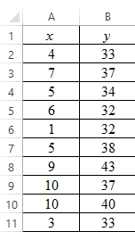
Sociology: Job Changes A sociologist is interested in the relation between x = number of job changes and y = annual salary (in thousands of dollars) for people living in the Nashville area. A random sample of 10 people employed in Nashville provided the following information:
| x (Number of job changes) | 4 | 7 | 5 | 6 | 1 | 5 | 9 | 10 | 10 | 3 |
| y (Salary in $1000) | 33 | 37 | 34 | 32 | 32 | 38 | 43 | 37 | 40 | 33 |
Complete parts (a) through (c), given
(d) If someone had x= 2 job changes, what does the least-squares line predict for y, the annual salary?
(a)
To graph: The scatter diagram.
Explanation of Solution
Given: The data which consists of variables, ‘number of job changes’ and ‘annual salary (in thousads of dollars)’, represented by x and y, respectively, is provided.
Graph:
Follow the steps given below in Excel to obtain the scatter diagram of the data.
Step 1: Enter the data into Excel sheet. The screenshot is given below.
Step 2: Select the data and click on ‘Insert’. Go to charts and select the chart type ‘Scatter’.
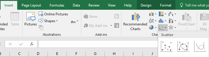
Step 3: Select the first plot and then click ‘add chart element’ provided on the left corner of the menu bar. Insert the ‘Axis titles’ and ‘Chart title’. The scatter plot for the provided data is shown below:
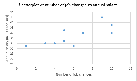
Interpretation: The scatter plot shows that there is a positive correlation between number of job changes and annual salary.
(b)
To find: The values of
Answer to Problem 10CR
Solution: The calculated values are
Explanation of Solution
Given: The provided values are
Calculation:
The value of
The value of
The value of
Therefore, the values are
The general formula for the least-squares line is,
Here, a is the y-intercept and b is the slope.
The value of
Substitute the values of a and b in the general equation to get the least-squares line of the data. That is,
Therefore, the least-squares line is
Follow the steps given below in Excel to obtain the least-squares line on the scatter diagram.
Step 1: Enter the data into Excel sheet. The screenshot is given below.
Step 2: Select the data and click on ‘Insert’. Go to charts and select the chart type ‘Scatter’.
Step 3: Select the first plot and then click ‘add chart element’ provided on the left corner of the menu bar. Insert the ‘Axis titles’ and ‘Chart title’. The scatter plot for the provided data is shown below:
Step 4: Right click on any data point and select ‘Add Trend line’. A dialogue box will open, select ‘linear’ and check ‘Display Equation on Chart’.
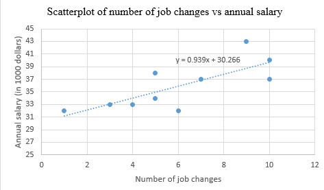
Interpretation: The scatter plot displays the equation of the least-squares line,
(c)
The values of r and
Answer to Problem 10CR
Solution: The values of r and
Explanation of Solution
Given: The provided values are
Calculation: The value of
Substitute the values in the above formula. Thus,
The coefficient of determination
Therefore, the value of
The value of
Interpretation: The correlation coefficient value
(d)
To find: The least-squares line forecast for y at
Answer to Problem 10CR
Solution: The forecasted value is $32,144.
Explanation of Solution
Given: The least-squares line from part (b) is
Calculation:
The predicted value
Thus, the value of
As the values of y are in 1000 dollars,
Interpretation: For a person who had 2 job changes, the predicted value of the annual salary using the least-squares line is $32144.
Want to see more full solutions like this?
Chapter 4 Solutions
Understanding Basic Statistics


 MATLAB: An Introduction with ApplicationsStatisticsISBN:9781119256830Author:Amos GilatPublisher:John Wiley & Sons Inc
 Probability and Statistics for Engineering and th...StatisticsISBN:9781305251809Author:Jay L. DevorePublisher:Cengage Learning
 Statistics for The Behavioral Sciences (MindTap C...StatisticsISBN:9781305504912Author:Frederick J Gravetter, Larry B. WallnauPublisher:Cengage Learning
 Elementary Statistics: Picturing the World (7th E...StatisticsISBN:9780134683416Author:Ron Larson, Betsy FarberPublisher:PEARSON
 The Basic Practice of StatisticsStatisticsISBN:9781319042578Author:David S. Moore, William I. Notz, Michael A. FlignerPublisher:W. H. Freeman
 Introduction to the Practice of StatisticsStatisticsISBN:9781319013387Author:David S. Moore, George P. McCabe, Bruce A. CraigPublisher:W. H. Freeman