
Statistics for Engineers and Scientists
4th Edition
ISBN: 9780073401331
Author: William Navidi Prof.
Publisher: McGraw-Hill Education
expand_more
expand_more
format_list_bulleted
Videos
Textbook Question
Chapter 7.4, Problem 14E
The article “Characteristics and Trends of River Discharge into Hudson, James, and Ungava Bays, 1964–2000” (S. Déry, M. Stieglitz, et al., Journal of Climate, 2005:2540–2557) presents measurements of discharge rate x (in km3/yr) and peak flow y (in m3/s) for 42 rivers that drain into the Hudson, James, and Ungava Bays. The data are shown in the following table:
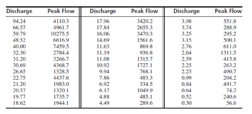
- a. Compute the least-squares line for predicting y from x. Make a plot of residuals versus fitted values.
- b. Compute the least-squares line for predicting y from ln x. Make a plot of residuals versus fitted values.
- c. Compute the least-squares line for predicting ln y from ln x. Make a plot of residuals versus fitted values.
- d. Which of the three models (a) through (c) fits best? Explain.
- e. Using the best model, predict the peak flow when the discharge is 50.0 km3/yr.
- f. Using the best model, find a 95% prediction interval for the peak flow when the discharge is 50.0 km3/yr.
Expert Solution & Answer
Want to see the full answer?
Check out a sample textbook solution
Students have asked these similar questions
An article in the ASCE Journal of Energy Engineering [“Overview of Reservoir Release Improvements at 20 TVA Dams” (Vol. 125, April 1999, pp. 1–17)] presents data on dissolved oxygen concentrations in streams below 20 dams in the Tennessee Valley Authority system. The observations are (in milligrams per liter):
An article in the Journal of Environmental Engineering (1989, Vol. 115(3), pp.
608–619) reported the results of a study on the occurrence of sodium and chloride in surface
streams in central Rhode Island. The following data are chloride concentration y (in milligrams per
liter) and roadway area in the watershed x (in percentage).
An article in the Journal of Applied Polymer Science (Vol. 56, pp. 471–476, 1995) studied the effect of the mole ratio of sebacic acid on the intrinsic viscosity of copolyesters.- The data follows: Viscosity 0.45 0.2 0.34 0.58 0.7 0.57 0.55 0.44 Mole ratio 1 0.9 0.8 0.7 0.6 0.5 0.4 0.3 (a) Construct a scatter diagram of the data.
Chapter 7 Solutions
Statistics for Engineers and Scientists
Ch. 7.1 - Compute the correlation coefficient for the...Ch. 7.1 - For each of the following data sets, explain why...Ch. 7.1 - For each of the following scatterplots, state...Ch. 7.1 - True or false, and explain briefly: a. If the...Ch. 7.1 - In a study of ground motion caused by earthquakes,...Ch. 7.1 - A chemical engineer is studying the effect of...Ch. 7.1 - Another chemical engineer is studying the same...Ch. 7.1 - Tire pressure (in kPa) was measured for the right...Ch. 7.1 - Prob. 10ECh. 7.1 - The article Drift in Posturography Systems...
Ch. 7.1 - Prob. 12ECh. 7.1 - Prob. 13ECh. 7.1 - A scatterplot contains four points: (2, 2), (1,...Ch. 7.2 - Each month for several months, the average...Ch. 7.2 - In a study of the relationship between the Brinell...Ch. 7.2 - A least-squares line is fit to a set of points. If...Ch. 7.2 - Prob. 4ECh. 7.2 - In Galtons height data (Figure 7.1, in Section...Ch. 7.2 - In a study relating the degree of warping, in mm....Ch. 7.2 - Moisture content in percent by volume (x) and...Ch. 7.2 - The following table presents shear strengths (in...Ch. 7.2 - Structural engineers use wireless sensor networks...Ch. 7.2 - The article Effect of Environmental Factors on...Ch. 7.2 - An agricultural scientist planted alfalfa on...Ch. 7.2 - Curing times in days (x) and compressive strengths...Ch. 7.2 - Prob. 13ECh. 7.2 - An engineer wants to predict the value for y when...Ch. 7.2 - A simple random sample of 100 men aged 2534...Ch. 7.2 - Prob. 16ECh. 7.3 - A chemical reaction is run 12 times, and the...Ch. 7.3 - Structural engineers use wireless sensor networks...Ch. 7.3 - Prob. 3ECh. 7.3 - Prob. 4ECh. 7.3 - Prob. 5ECh. 7.3 - Prob. 6ECh. 7.3 - The coefficient of absorption (COA) for a clay...Ch. 7.3 - Prob. 8ECh. 7.3 - Prob. 9ECh. 7.3 - Three engineers are independently estimating the...Ch. 7.3 - In the skin permeability example (Example 7.17)...Ch. 7.3 - Prob. 12ECh. 7.3 - In a study of copper bars, the relationship...Ch. 7.3 - Prob. 14ECh. 7.3 - In the following MINITAB output, some of the...Ch. 7.3 - Prob. 16ECh. 7.3 - In order to increase the production of gas wells,...Ch. 7.4 - The following output (from MINITAB) is for the...Ch. 7.4 - The processing of raw coal involves washing, in...Ch. 7.4 - To determine the effect of temperature on the...Ch. 7.4 - The depth of wetting of a soil is the depth to...Ch. 7.4 - Good forecasting and control of preconstruction...Ch. 7.4 - The article Drift in Posturography Systems...Ch. 7.4 - Prob. 7ECh. 7.4 - Prob. 8ECh. 7.4 - A windmill is used to generate direct current....Ch. 7.4 - Two radon detectors were placed in different...Ch. 7.4 - Prob. 11ECh. 7.4 - The article The Selection of Yeast Strains for the...Ch. 7.4 - Prob. 13ECh. 7.4 - The article Characteristics and Trends of River...Ch. 7.4 - Prob. 15ECh. 7.4 - The article Mechanistic-Empirical Design of...Ch. 7.4 - An engineer wants to determine the spring constant...Ch. 7 - The BeerLambert law relates the absorbance A of a...Ch. 7 - Prob. 2SECh. 7 - Prob. 3SECh. 7 - Refer to Exercise 3. a. Plot the residuals versus...Ch. 7 - Prob. 5SECh. 7 - The article Experimental Measurement of Radiative...Ch. 7 - Prob. 7SECh. 7 - Prob. 8SECh. 7 - Prob. 9SECh. 7 - Prob. 10SECh. 7 - The article Estimating Population Abundance in...Ch. 7 - A materials scientist is experimenting with a new...Ch. 7 - Monitoring the yield of a particular chemical...Ch. 7 - Prob. 14SECh. 7 - Refer to Exercise 14. Someone wants to compute a...Ch. 7 - Prob. 16SECh. 7 - Prob. 17SECh. 7 - Prob. 18SECh. 7 - Prob. 19SECh. 7 - Use Equation (7.34) (page 545) to show that 1=1.Ch. 7 - Use Equation (7.35) (page 545) to show that 0=0.Ch. 7 - Prob. 22SECh. 7 - Use Equation (7.35) (page 545) to derive the...
Additional Math Textbook Solutions
Find more solutions based on key concepts
z Scores. In Exercises 5-8, express all z scores with two decimal places.
8. Plastic Waste Data Set 31 “Garbage...
Elementary Statistics Using Excel (6th Edition)
How much time do Americans living in or near cities spend waiting in traffic, and how much does waiting in traf...
Business Statistics: A First Course (7th Edition)
The data in Table 1A were collected from one of the authors’ statistics classes. The first row gives the variab...
Introductory Statistics
Use the model developed in Example 1.5 to predict the total sales for weeks 2 through 16, and compare the resul...
Business Analytics
Testing Hypotheses. In Exercises 13-24, assume that a simple random sample has been selected and test the given...
Elementary Statistics Using the TI-83/84 Plus Calculator, Books a la Carte Edition (4th Edition)
Knowledge Booster


Learn more about
Need a deep-dive on the concept behind this application? Look no further. Learn more about this topic, statistics and related others by exploring similar questions and additional content below.Similar questions
- An article in Technometrics (1974, Vol. 16, pp. 523–531) considered the following stack-loss data from a plant oxidizing ammonia to nitric acid. Twenty-one daily responses of stack loss (the amount of ammonia escaping) were measured with air flow x1, temperature x2, and acid concentration x3. y = 42, 37, 37, 28, 18, 18, 19, 20, 15, 14, 14, 13, 11, 12, 8, 7, 8, 8, 9, 15, 15 x1 = 80, 80, 75, 62, 62, 62, 62, 62, 58, 58, 58, 58, 58, 58, 50, 50, 50, 50, 50, 56, 70 x2 = 27, 27, 25, 24, 22, 23, 24, 24, 23, 18, 18, 17, 18, 19, 18, 18, 19, 19, 20, 20, 20 x3 = 89, 88, 90, 87, 87, 87, 93, 93, 87, 80, 89, 88, 82, 93, 89, 86, 72, 79, 80, 82, 91 (a) Fit a linear regression model relating the results of the stack loss to the three regressor variables. (b) Estimate σ2. (c) Find the standard error se(βj). (d) Use the model in part (a) to predict stack loss when x1 = 60, x2 = 26, and x3 = 85.arrow_forwardrofessor Cornish studied rainfall cycles and sunspot cycles. (Reference: Australian Journal of Physics, Vol. 7, pp. 334-346.) Part of the data include amount of rain (in mm) for 6-day intervals. The following data give rain amounts for consecutive 6-day intervals at Adelaide, South Australia. 7 28 7 1 69 3 1 4 22 7 16 4 54 160 60 73 27 3 3 1 7 144 107 4 91 44 1 8 4 22 4 59 116 52 4 155 42 24 11 43 3 24 19 74 26 63 110 39 34 71 52 39 8 0 15 2 14 9 1 2 4 9 6 10 (i) Find the median. (Use 1 decimal place.)(ii) Convert this sequence of numbers to a sequence of symbols A and B, where A indicates a value above the median and B a value below the median. Test the sequence for randomness about the median at the 5% level of significance. (b) Find the number of runs R, n1, and n2. Let n1 = number of values above the median and n2 = number of values below the median. R n1 n2 (c) In the case, n1 > 20, we cannot use Table 10 of Appendix II to find the critical…arrow_forwardAn article in the Fire Safety Journal (“The Effect of Nozzle Design on the Stability and Performance of Turbulent Water Jets,” Vol. 4, August 1981) describes an experiment in which a shape factor was determined for several different nozzle designs at six levels of jet efflux velocity. Interest focused on potential differences between nozzle designs (blocks), with velocity considered as a nuisance variable. The data are shown below: Jet Efflux Velocity (m/s) Nozzle Design 11.73 14.37 16.59 20.43 23.46 28.74 1 0.78 0.80 0.81 0.75 0.77 0.78 2 0.85 0.85 0.92 0.86 0.81 0.83 3 0.93 0.92 0.95 0.89 0.89 0.83 4 1.14 0.97 0.98 0.88 0.86 0.83 5 0.97 0.86 0.78 0.76 0.76 0.75 1) Write the null hypothesis and the alternative hypothesis (for the factor). 2) Find the ANOVA table. (round to five decimal places). 3) What is your decision about the null hypothesis, consider ?. 4) If your decision in part (4) was reject , perform Tukey test to determine which pairwise means are…arrow_forward
- ) The following table shows 10 communities ranked by decayed, missing, or filled (DMF) teeth per 100 children and fluoride concentration in ppm in the public water supply: Rank by DMF Teeth FluorideCommunity per 100 children X Concentration Y 1 8 1 2 9 3 3 7 4 4 3 9 5 2 8 6 4 77 1…arrow_forwardThe following partial JMP regression output for the Fresh detergent data relates to predicting demand for future sales periods in which the price difference will be .10. SE Fit = .165360573, s = .628152. Predicted Demand Lower 95% MeanDemand Upper 95% MeanDemand 31 8.181072245 7.842346262 8.519798229 StdErr IndivDemand Lower 95% IndivDemand Upper 95% MeanDemand 0.649552965 6.850522511 9.511621980 Click here for the Excel Data File (a) Report a point estimate of and a 95 percent confidence interval for the mean demand for Fresh in all sales periods when the price difference is .10. (Round your CI answers to 3 decimal places and other answer to 4 decimal places.) (b) Report a point prediction of and a 95 percent prediction interval for the actual demand for Fresh in an individual sales period when the price difference is .10. (Round your PI answers to 3 decimal places and other answer to 4 decimal places.) (c) StdErr Indiv Demand on…arrow_forwardThe Turbine Oil Oxidation Test (TOST) and the Rotating Bomb Oxidation Test (RBOT) are two different procedures for evaluating the oxidation stability of steam turbine oils. An article reported the accompanying observations on x = TOST time (hr) and y = RBOT time (min) for 12 oil specimens. TOST 4200 3600 3750 3650 4050 2770 RBOT 370 345 375 315 350 205 TOST 4870 4525 3450 2700 3750 3325 RBOT 400 380 285 220 345 290 (a) Calculate the value of the sample correlation coefficient. (Round your answer to four decimal places.) r = Carry out a test of hypotheses to decide whether RBOT Time and TOST time are linearly related. (Use ? = 0.05.) Calculate the test statistic and determine the P-value. (Round your test statistic to two decimal places and your P-value to three decimal places.) t = P-value =arrow_forward
- In Applied Life Data Analysis (Wiley, 1982), Wayne Nelson presents the breakdown time of an insulating fluid between electrodes at 34 kV. The times, in minutes, are as follows: 0.19, 0.78, 0.96, 1.31, 2.78, 3.16, 4.15, 4.67, 4.85, 6.50, 7.35, 8.01, 8.27, 12.06, 31.75, 32.52, 33.91, 36.71, and 72.89. Calculate the sample mean and sample standard deviation.arrow_forwardSample data on weekly sales of two dairy products, X and Y were reported as follows: Lilongwe dairy, X 120 100 160 250 180 130 300 40 Long life, Y 70 86 67 100 45 80 90 95 a. Apply the CV, and find out which of the 2 products shows greater fluctuations in sales.arrow_forwardHow sensitive to changes in water temperature are coral reefs? To find out, scientists examined data on sea surface temperatures, in degrees Celsius, and mean coral growth, in centimeters per year, over a several‑year period at locations in the Gulf of Mexico and the Caribbean Sea. The table shows the data for the Gulf of Mexico. Sea surface temperature 26.726.7 26.626.6 26.626.6 26.526.5 26.326.3 26.126.1 Growth 0.850.85 0.850.85 0.790.79 0.860.86 0.890.89 0.920.92 (b) Find the correlation ?r step by step. Round off to two decimals places in each step. First, find the mean and standard deviation of each variable. Then, find the six standardized values for each variable. Finally, use the formula for ?r . Round your answer to three decimal places.arrow_forward
- Following are measurements of soil concentrations (in mg /kg) of chromium (Cr) and nickel (Ni) at20 sites in the area of Cleveland, Ohio. These data are taken from the article "Variation in NorthAmerican Regulatory Guidance for Heavy Metal Surface Soil Contamination at Commercial andIndustrial Sites" (A. Jennings and J. Ma, J. Environment Eng, 2007:587-609). Cr: 260 19 36 247 263 319 317 277 319 264 23 29 61 119 33 281 21 35 64 30Ni: 435 377 359 53 38 38 54 188 397 33 92 490 28 35 799 347 321 32 74 508 (a) Construct a histogram for each set of concentrations. (b) Find the 1st, 2nd and 3rd quartiles for the Cr concentrations (c) Find the 1st, 2nd and 3rd quartiles for the Ni concentrations.arrow_forwardThe data given is shown below 40 40 43 46 44 49 51 54 46 51 47 49 49 45 45 44 45 41 49 52 51 54 50 51 41 52 53 50 46 56 42 42 40 42 49 47 51 48 46 57 48 55 49 46 57 44 49 43 44 43 51 48 48 46 49 Class width = 6 Find the following: A. Decile (5th) B. Quartile (2nd) C. Skewness D. Kurtosisarrow_forwardIn the article “Groundwater Electromagnetic Imaging in Complex Geological and Topographical Regions: A Case Study of a Tectonic Boundary in the French Alps” (S. Houtot, P. Tarits, et al., Geophysics, 2002:1048–1060), the pH was measured for several water samples in various locations near Gittaz Lake in the French Alps. The results for 11 locations on the northern side of the lake and for 6 locations on the southern side are as follows: Northern side: 8.1 8.2 8.1 8.2 8.2 7.4 7.3 7.4 8.1 8.1 7.9 Southern side: 7.8 8.2 7.9 7.9 8.1 8.1 Find a 98% confidence interval for the difference in pH between the northern and southern side.arrow_forward
arrow_back_ios
SEE MORE QUESTIONS
arrow_forward_ios
Recommended textbooks for you
 Glencoe Algebra 1, Student Edition, 9780079039897...AlgebraISBN:9780079039897Author:CarterPublisher:McGraw Hill
Glencoe Algebra 1, Student Edition, 9780079039897...
Algebra
ISBN:9780079039897
Author:Carter
Publisher:McGraw Hill
Hypothesis Testing using Confidence Interval Approach; Author: BUM2413 Applied Statistics UMP;https://www.youtube.com/watch?v=Hq1l3e9pLyY;License: Standard YouTube License, CC-BY
Hypothesis Testing - Difference of Two Means - Student's -Distribution & Normal Distribution; Author: The Organic Chemistry Tutor;https://www.youtube.com/watch?v=UcZwyzwWU7o;License: Standard Youtube License